Circular 688
Louis C. Bender
College of Agricultural, Consumer and Environmental Sciences
Author: Senior Research Scientist (Natural Resources), Department of Extension Animal Sciences and Natural Resources, New Mexico State University. (Print Friendly PDF)
Summary
Predation is a much misunderstood ecological process. Most people confuse the act of predation with the effect, believing that the killing of an individual animal invariably results in a negative impact on the population (Figure 1). This view is frequently wrong, and ignores the complexity of predation at the individual, population, and community levels. At the individual level, predisposition refers to characteristics (e.g., poor body condition, inadequate cover, disease, etc.) of individuals that make them more or less likely to die from predation or any other cause. Predisposition influences whether (or how likely it was that) an individual would have lived if not killed by a predator. The greater the degree of predisposition, the less likely the death of a predated individual would have any effect on the population. Predisposition is necessary for predation to be compensatory, or substitutive, at the level of the population. Compensatory mortality means that instead of adding additional mortality to the population (i.e., additive mortality), increases in predation result in compensatory declines in other causes of mortality. Hence, the overall survival rate of the population is not decreased, so predation has little effect on the population. Communities in turn are affected by whether predation is primarily compensatory or additive because high levels of additive predation can destabilize communities. Highlighting this complexity, few examples exist of predator control having any positive effect on prey populations in the Southwest. Confusion also comes from predator-prey investigations; most do little more than simply identify causes of death of prey, which says nothing of the effect of predation on prey. Unreliable or no assessment of predisposition of prey, or using simplistic models (such as predator:prey ratios) to infer predation effects, similarly contribute to misinformed views of predation. Consequently, both the general public and professional biologists often have a poor understanding of how, why, and to what degree, if any, predation actually affects prey populations.
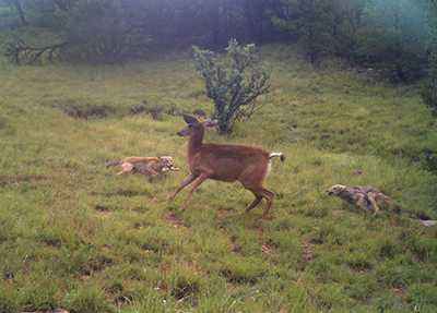
Figure 1. Predation is a frequently misunderstood ecological process, primarily because people empathize with the prey and confuse the act of predation with the effect of predation on populations of prey. While successful predation results in the death of individuals, those deaths may have little or no effect on the population as a whole. (Photo courtesy of L. Bender.)
Introduction
Many people, including professional wildlife biologists, lack a clear understanding of the role of predation in wildlife populations. This results from a natural confusion regarding the act of predation (i.e., the killing of an individual) and the effect of predation (i.e., does predation affect population size?) (Errington, 1946, 1967). Most biologists are also taught predator-prey interactions using simple theoretical models (i.e., Lotka-Volterra and subsequent derivations; Hassel, 1978; Begon and Mortimer, 1981; Sinclair and Pech, 1996), which invariably assume that predation decreases the prey population size if any individuals are killed. Further, simplistic measures, such as predator:prey ratios, are often believed to predict the effect of predators on prey populations, despite the known unreliability of such approaches (Theberge, 1990; Bowyer et al., 2013). However, probably the most important issue contributing to the lack of understanding of predator-prey interactions is a lack of appreciation for the complexities that determine the effect of predation on prey populations.
In reality, the interactions of predators and prey are far from clear-cut. What we can safely generalize about predation is that predators can and do impact prey populations under certain circumstances. Under other circumstances, predation has little or no effect on prey populations, even though it may be the main cause of death for individuals in those populations. What determines the outcome are the local ecological conditions, which can vary greatly with regards to habitat characteristics, numbers of predator species, numbers and vulnerability of prey, population age structure, weather, and hunting behavior of predators, among many others (Errington, 1967; National Research Council, 1997; Ballard and Van Ballenberghe, 1998; Heffelfinger, 2006; Wilmers et al., 2007; Bender, 2008; Mech, 2012; Sinclair, 2003; Forrester and Wittmer, 2013; Bowyer et al., 2013; Bender and Rosas-Rosas, 2016). Predation is also hierarchical, meaning that it acts at multiple levels, including the individual, the population, and the community or ecosystem. Appreciating how predation acts on each of these, and how the impacts of predation, if any, flow up through these levels, is key to understanding this complex ecological phenomenon.
The Hierarchy of Predation
Predation acts on three levels, starting with the individual and working up to the community through its effects on populations (Figure 2). At each of these levels, different processes are at work. The key issue at the level of the individual is predisposition; in other words, are certain individuals predisposed to death regardless of the cause? This influences the impact of predation at the level of the population, where predation can either be compensatory or additive to varying degrees. This determines whether predation mainly substitutes for other mortality factors or adds to total mortality experienced by the population, or whether the population reacts in some other manner, such as by increasing productivity. The location along the compensatory-additive continuum usually determines the effect of predation at the community level: Does predation help to stabilize or destabilize the system? Each of these levels influences the level above, but predation may have differing implications at each level. Because of this, how predation functions at each level needs to be appreciated to understand how predation affects the entire system.
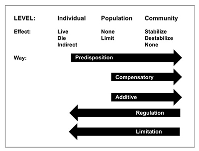
Figure 2. The hierarchy of predation. The direct effect of predation on individuals in a population is that an individual either lives or dies. Whether any particular individual lives or dies is related to their predisposition to mortality. The level of predisposition influences the effect of predation at the level of the population, where it either substitutes for other mortality factors (compensatory) or adds to them (additive). The greater the predisposition, the more likely predation is to be compensatory. At the community level, compensatory mortality acts to stabilize communities by functioning as a regulatory (negative feedback) force, whereas additive mortality acts to destabilize communities.
Individuals
Individuals in a population are always dying from a variety of causes, including accidents, disease, malnutrition, hunter harvest, predation, and old age, to name only a few. Because of that, survival is never 100% in a population; a certain proportion of the population (the annual mortality) is always lost. The proportion lost depends upon many things, chiefly the quality of habitat in terms of providing food and/or cover. As habitat quality declines, mortality increases because more individuals die. In a world completely free of predators, disease, and bad luck, a proportion of each population would still die each year, and that proportion is roughly equal to the inverse of the species life span. For example, if a species can live about 20–25 years, like elk (Cervus elaphus), the minimum level of mortality annually would be about 4–5% (Bender, 2013). This is termed “chronic mortality.” Only when the number of individual deaths in a population rises above this background level can predation or any other mortality factor become a relevant variable in population dynamics.
The direct effect of predation at the level of the individual is that an individual is either killed by a predator or not (potential indirect effects of predation are addressed below). Whether that individual is killed or not often depends upon its degree of predisposition. In other words, is there some characteristic of that individual that makes it more or less likely to be killed by a predator? Many factors can predispose individuals to predation or any other cause of death. For larger animals, perhaps the most important of these is nutritional or body condition (Hanks, 1981; Mech and Peterson, 2003; Bender and Rosas-Rosas, 2016). Individuals in poor shape are more vulnerable for many reasons, including less ability to fight or flee, less environmental awareness and hence less ability to detect the presence of a predator, greater susceptibility to disease and accidents, etc. Other traits can also predispose individuals to predation, including age, debilitation (i.e., injury), and diseases such as chronic wasting disease (CWD) (Errington, 1967; Mech and Peterson, 2003; Mech, 2012; Krumm et al., 2010). For example, CWD decreases individual condition and reduces environmental awareness. Consequently, CWD has been shown to predispose mule deer (Odocoileus hemionus) to predation and to deer-vehicle collisions (Krumm et al., 2005, 2010). Similar, predators such as wolves (Canis lupus) often kill aged or injured large prey (Mech and Peterson, 2003; Mech, 2012), and these individuals may contribute little to population growth (Bender and Hoenes, 2017).
Climatic conditions can also predispose individuals (Mech and Peterson, 2003; Bender et al., 2013; Bender and Rosas-Rosas, 2016). Most relevant for New Mexico, drought can lower condition of individuals by decreasing forage quality regardless of the number of individuals present or the quantity of forage available (DeYoung et al., 2000; Bender and Cook, 2005; Bender and Rosas-Rosas, 2016). Similarly, adverse weather such as deep snow can reduce condition of prey, increasing predisposition of individuals (Ballard and Van Ballenberghe, 1998; Mech and Peterson, 2003).
Some conditions that may increase vulnerability of prey do not necessarily increase predisposition of prey, however. For example, drought can also force individuals to congregate around a limited number of water sites, making them easier for predators to locate, and making detection of, and escape from, predators more difficult (Polisar et al., 2003; Rosas-Rosas et al., 2008, 2010). Similarly, deep snow can limit the ability of prey to run from predators, which are often smaller and able to run on crusted snow where prey break through (Ballard and Van Ballenberghe, 1998; Mech and Peterson, 2003). Such conditions increase vulnerability to predation, but they would only increase predisposition of individuals if they also increased the likelihood of death from other mortality factors.
Human actions can also increase vulnerability, and potentially predisposition, of prey. For example, laissez faire livestock management may result in increased livestock-predator interactions around water sites, increasing vulnerability and facilitating predation (Rosas-Rosas et al., 2008, 2010). Co-occurrence of livestock and wildlife may also facilitate disease transmission to wildlife (and vice versa), resulting in debilitation and increased predisposition (e.g., Krausman et al., 1996).
Small and large species can also differ with respect to predisposing mechanisms. The life history strategy of large mammals (K-selection) emphasizes maximizing adult survival rather than overproduction of young (Begon and Mortimer, 1981), so condition is the most common mechanism through which predisposition operates. Small species like upland game birds emphasize overproduction of young (i.e., are r-selected; Errington, 1967; Begon and Mortimer, 1981). This overproduction is often termed a ”doomed surplus” (Errington, 1967; Boyce et al., 1999) because the vast majority of these individuals will die, regardless of the cause. These r-selected species are most commonly limited by the availability of cover; sufficient high-quality security cover is usually available for only a certain number of individuals, and the remainder, primarily the “overproduced young,” are highly predisposed and most or all will die under typical conditions (Errington, 1967). Why? Those produced over the habitat’s “threshold for security” are highly vulnerable to most causes of mortality, including severe weather and predation (Errington, 1967). In other words, there is usually simply no space for them.
The most common precept of predisposition is that a certain minimum level of condition (or available cover within a home range; for example, sufficient residual grass or shrub cover to roost under [Errington, 1967]) exists below which individuals are not viable (meaning that they would likely die regardless of proximate cause; Errington, 1967; Bender and Rosas-Rosas, 2016), or that individuals become increasingly predisposed to death as condition declines. This highlights the importance of differentiating between proximate and ultimate causes of death (Bender and Rosas-Rosas, 2016). The proximate cause of death is what caused the individual to die at that moment (i.e., what “struck the final blow”), whereas the ultimate cause of death is what was truly responsible for the loss of the individual. To illustrate, a puma (Puma concolor) may kill a mule deer that is completely unaware of its environment because of a disease such as CWD. Here, the predator was the proximate cause of death (i.e., it “struck the final blow”) but the individual would have invariably died shortly from some other factor (or to some other predator) because the disease had eliminated its ability to survive. Hence, the ultimate cause was disease; the deer would have died regardless of who or what “struck the final blow.” Unfortunately, many studies of survival of wildlife do little beyond listing a proximate cause of death. Such studies contribute little to understanding predation beyond simply identifying things that could possibly kill an animal (Bender and Rosas-Rosas, 2016), even if they include some index of population trend. They do not determine the effect of predation or any other mortality factor on populations, do not test for other environmental factors affecting populations, and thus should not be used to assess the effect of predation on prey (Bender and Rosas-Rosas, 2016).
It is important to understand that predisposition can be both relative and absolute in populations. Relative predisposition affects individuals that are in poorer condition than the population as a whole. For example, all mule deer killed by pumas were in poorer condition than their population as a whole in several New Mexico studies (Bender and Rosas-Rosas, 2016). Further, these populations as a whole were in very poor condition (e.g., lactating females averaged <6% body fat, about 1/3 of levels indicative of excellent condition; Bender et al., 2011), and thus all individuals were likely predisposed to some degree (Bender and Rosas-Rosas, 2016). This illustrates absolute predisposition, which affects all individuals in the population, and is present when the population as a whole is in poor condition. For example, of 371 adult female elk that I captured and assessed for condition in the arid and semi-arid West and Mexico, only 10 (2.6%) were in excellent condition (i.e., >16% body fat; Cook et al., 2004) and just 124 (33.4%) were in good condition (>12% body fat; Cook et al., 2004) at the seasonal peak of condition. The vast majority of individuals in these populations were thus predisposed to mortality to some degree because of the low overall condition of these populations.
The above discussion has emphasized the direct effect of predation on individuals. Predation, however, can indirectly affect individuals (and populations) as well. For example, the presence of predators may change the distribution and/or habitat use patterns of prey (e.g., Hernandez and Laundre, 2005; Gude et al., 2006). This, in turn, could result in decreased condition of individuals because of the use of poorer habitats, or result in increased disturbance of prey populations (Hernandez and Laundre, 2005). Both of these indirect effects can reduce individual- and population-level productivity (Phillips and Alldredge, 2000), and thus the population’s potential rate of increase. While such effects are often described in predator-prey studies, how common they are and the actual role of predators in them remains uncertain (Mech, 2012).
To summarize, the act of predation occurs at the individual level. The direct effect, at this level, is the death of an individual. The mechanism that can influence whether any particular individual lives or dies is predisposition (Figure 3). The important question is whether, or how likely it was that, they would have lived if not killed by that predator (or other factor). The greater the degree of predisposition, the less likely the death of the individual would have any effect on the population. Thus, the degree of predisposition drives the effect of predation at the next level, the level of the population.
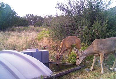
Figure 3. Most people, including many biologists, believe that all attacks by a predator are invariably successful. The reality is that predators are far from perfect. Although it cannot be known with certainty, the nature and location of the wounds suggest that it is highly likely that a puma tried to take down this young buck (right) and failed. (Photo courtesy of L. Bender.)
Population
Most conflicts associated with predation result from the perceived effects on the prey population. Effects of predation on populations fall along a continuum from compensatory to additive (Figure 4). If predation is primarily compensatory mortality, it has little effect on populations (Errington, 1967; Bartmann et al., 1992; Boyce et al., 1999). What compensatory means is substitutive. If mortality is compensatory, an increase in one cause of death or mortality factor like predation is “compensated” for by declines in other mortality factors, such as starvation (Figure 5). The reverse is also true; if predation declines, other mortality factors such as starvation or disease would increase. As a result, the total mortality level of the population remains about the same, but the number of losses to any cause of mortality may change dramatically, albeit out of phase with each other (i.e., if one increases, the others decline). Therefore, in the case of compensatory mortality, an increasing predation rate has little effect on the survival rate of the prey (Figures 4 and 5) because mortality is compensated for or “traded” among causes.
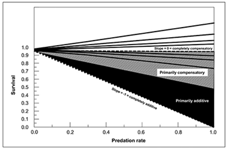
Figure 4. The effect of increasing predation rate on the survival rate of individuals in a population determines whether predation is additive or compensatory mortality. If totally additive, each increase in predation would result in an equal decrease in survival. For example, a predation rate of 0.2 would decrease survival from 1.0 to 0.8. Thus, total additivity is characterized by a corrected slope of −1 (lower dashed line). If completely compensatory, then any increase in predation rate would have no influence on survival, resulting in a corrected slope of 0 (middle dashed line). Between these two extremes is a slope of −0.5, above which predation is primarily compensatory (light shading) and below which predation is primarily additive (dark shading). Plotted are all data (solid lines) from regressions of arcsin-squareroot transformed predation and survival rates from populations of mule deer, elk, pronghorn, and desert bighorn sheep that have explicitly tested this relationship (Bender and Rosas-Rosas, 2016; Bender et al., 2017; L. Bender, unpublished data). Note that all corrected slopes plot in the mostly to completely compensatory region (i.e., slopes >−0.50).
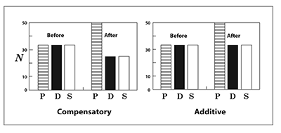
Figure 5. Illustrating compensatory and additive mortality resulting from a 50% increase in numbers of predation mortalities. In each case, prior to the increase in predation the population loses 33 individuals each to predation (P), disease (D), and starvation (S). In the compensatory case, the predation mortality increases to 50 individuals, while disease and starvation decrease to 25 individuals each. The increase in predation is compensated for by declines in disease and starvation, and thus total mortality remains unchanged at around 100 individuals. In the additive case, the increase in predation does not result in any declines in disease and/or starvation, so total mortality increases from around 100 individuals to around 117. In this case, the increase in predation has added additional mortality to the population.
At the opposite end of this continuum is additive mortality. If mortality is additive, it adds additional mortality on top of existing mortality (Errington, 1967; Bartmann et al., 1992). As a result, the total mortality of a population increases, and the overall survival rate declines (Figures 4 and 5). It is when predation or other mortality factors become additive that they can limit a population, i.e., they “limit” the potential population rate of increase or size to some level lower than it would be in the absence of that mortality factor. Thus, the important question regarding predation at the population level is: to what degree is it additive or compensatory? Predation or any other mortality factor is usually never completely compensatory or additive; rather, it falls somewhere along the continuum between the two (Figure 4). Where exactly it falls along the continuum determines its effect on populations, and whether this effect is large enough to even be detected.
For predation to be compensatory, some degree of predisposition must be present at the individual level (Bender and Rosas-Rosas, 2016). The more predisposed individuals are, the more likely predation is to be compensatory. For example, individuals in a severely overpopulated population, during a drought, or on poor range are invariably in very poor condition, and many will die from various causes, including disease, starvation, or within-species fights. It does not matter what these individuals die from—disease, starvation, predation, or any other factor—because a certain percentage of individuals will die regardless. In other words, if a predator does not “strike the final blow” for individual X, then there is a high probability that disease or starvation will. Why? Because some or all individuals in that population are strongly predisposed to mortality (i.e., have significantly increased probability of dying).
Predisposition can similarly act on species capped by the amount of suitable cover. If suitable security cover is available for only 100 individuals, then any individuals above that number have little chance of surviving through the season of limitation, usually overwinter. It does not matter whether predators kill all or none of this “doomed surplus” because these individuals would in all likelihood not survive regardless (Errington, 1967; Boyce et al., 1999).
The degree of predisposition is often the key factor that differentiates predation on wildlife from predation on livestock. Unlike livestock, wildlife do not receive vaccinations against diseases, veterinary care if sick, etc. Because of these livestock management practices, mortality in adult livestock seldom exceeds chronic minimums, and thus there is little opportunity under most conditions for compensation to operate, since there is little extra mortality above the chronic minimum to “trade” among causes of death. That is not always the case, however. Maternal care is frequently much less intensive in livestock as compared to wildlife, and thus mortality of juveniles has a greater chance to be compensatory (Rosas-Rosas et al., 2008).
Compensatory and additive mortality
This leads to the most common misconception people have regarding predation, namely that the individual killed by the predator would still be alive if the predator was removed. This simplistic view is used, for example, to justify many predator control programs, and ignores the concepts of predisposition and compensatory mortality. Simply, if predisposition is present, the individual killed by the predator was likely to have died from some other cause anyway. To illustrate, research in New Mexico has shown that individual mule deer killed by pumas were in significantly poorer condition than the population as a whole (Bender and Rosas-Rosas, 2016). This illustrates predisposition; such individuals were increasingly likely to die from some other factor if not killed by a puma. Hence, mortality in these populations was primarily compensatory (Figure 4; Bender and Rosas-Rosas, 2016). Primarily compensatory predation was similarly seen with pronghorn (Antilocapra americana), elk, and desert bighorn (Ovis canadensis) across multiple populations in New Mexico (Figure 4).
Conversely, if individuals in a population are not predisposed by poor condition, lack of cover, or other factors, predation can be much more of an additive mortality factor. Such circumstances can occur in high-quality habitats where individuals attain excellent nutrition, or in areas where there are multiple efficient predators of both juveniles and adults (if the prey species has multiple distinct age classes). In the case of high-quality habitat, individuals, especially adults, are likely at or near the chronic minimum levels of mortality. Because there is no additional mortality to “trade” among causes, any new mortality such as predation mostly adds to existing mortality under these circumstances. Interestingly, the response of the population to predation can still be compensatory to some degree under these circumstances if density dependence is the primary factor affecting population condition, but the method of compensation changes. Compensation in these cases can occur through an increase in the number of juveniles born (termed compensatory natality) and/or survival of juveniles (see Density dependence and population age structure, below; Bender, 2008, 2018).
Sometimes, even if individuals in a prey population are strongly predisposed, predation can still be mostly additive. These circumstances involve systems with multiple efficient large predators (especially social or pack predators) and vulnerable alternative prey species (National Research Council, 1997; Ballard and Van Ballenberghe, 1998). For example, combined predation on moose (Alces alces) by wolves, brown bears (Ursus arctos), and black bears (Ursus americanus) can limit moose populations in some areas where caribou (Rangifer tarandus) and other prey are also present. As moose decline, the large carnivores are able to shift to other vulnerable prey to maintain their own population size, but still preferentially utilize adult and calf moose, their preferred prey. Because the predators do not decline in population size nor does predation pressure on moose lessen, predators can limit the growth of moose populations. Such conditions can lead to a “predator-pit” or low-density equilibrium (Ballard and Van Ballenberghe, 1998), where the primary prey species is maintained at low density because of multiple species of efficient predators preying on both adults and juveniles in a depensatory (inversely density dependent) manner, meaning that predation pressure increases as the prey population declines (Figure 6).
Density dependence and population age structure
Much of the above has focused on compensatory or additive mortality within populations with approximately equal vulnerability among age classes, or within a specific age class, such as adult females. If present, other characteristics of populations, such as density dependence or having a complex age structure, can provide populations with additional mechanisms to compensate for predation beyond compensatory mortality within a population segment (Bender, 2008, 2018).
The population process called density dependence affects populations through the amount of resources available to individuals as a result of competition. Because resources (food, water, cover, space) are not unlimited, as the size of a population increases, the quantity and/or quality of resources available to individuals declines (Begon and Mortimer, 1981; Bender, 2011). This decline in per capita resource availability results in decreased condition and increased stress in individuals, the magnitude of which increases as population size increases and resource availability declines. This results in a slowing of the rate of population growth because of declining condition of adults and/or increasing stress. This slowing of population growth occurs primarily because of impacts on production and survival of young, although adult survival can also be affected (Gaillard et al., 2000). Why? Because resource stress affects individuals in a population in a fairly predictable order, i.e., first body condition declines, followed by lower juvenile fecundity and survival, then lower adult fecundity, and finally lower adult survival (Gaillard et al., 2000).
Not all populations experience strong density dependence. Many populations in the arid Southwest, for example, may never reach densities where strong competition occurs because populations are kept below this level by frequent drought or other density-independent effects that reduce productivity and survival (e.g., pronghorn [Bender et al., 2013]). Those populations that do show strong density dependence, however, have additional mechanisms to compensate for predation (or other causes of mortality). As noted above, increasing population density results in individuals finding less quality food (or fewer quality cover sites) and thus becoming increasingly predisposed because of poor condition or inadequate cover. Under the density-dependent case, at higher densities loss of an individual to a predator (or other cause of death) increases available resources for the remaining individuals (and thereby reduces predisposition and vulnerability). Thus, the degree (or strength) and timing of density dependence can be important in determining whether predation is additive or compensatory on populations (Errington, 1967; Boyce et al., 1999; Ballard et al., 2003). If strong density-dependent effects are occurring in populations, predation is more likely to be compensatory.
However, compensation in the case of strong density dependence can also occur through an increase in the number of juveniles born (compensatory natality) and/or survival of juveniles (Bender, 2008, 2018), in addition to compensatory mortality among adults. The reason is that production and survival of juveniles are affected by even minor levels of resource stress (Gaillard et al., 2000), and juveniles thus have greater potential to respond to increases in resource availability caused by decreased competition. In contrast, adult survival is the last population demographic affected by resource stress (Gaillard et al., 2000). Thus, under any degree of density-dependent resource limitation, a population has some ability to compensate for predation or other mortality, even if it is primarily additive for one component of the population, such as adults. Only under optimal nutrition and cover is that ability lost, and such conditions never occur in nature.
Many biologists mistakenly believe that compensatory responses can occur only if strong density dependence is working on a population. This belief is particularly unfortunate in arid environments such as New Mexico, where forage quality can be very low regardless of the abundance of forage. Thus, condition of individuals can be poor because of a density-independent effect (low forage quality) rather than density dependence. Such density-independent (meaning that it does not matter whether there are many or few individuals in a population) effects can also decrease condition and increase predisposition. Again, included here are things like drought that limit the availability of nutritious foods, or situations where the game range is in poor condition because of few quality foods as a result of past overutilization (DeYoung et al., 2000; Bender and Cook, 2005; Bender and Rosas-Rosas, 2016). In these cases, regardless of whether there are many or few individuals in the population (i.e., regardless of the degree of competition), each individual cannot attain good condition because the nutritional quality of the forage is simply inadequate (Bender and Cook, 2005).
For species like ungulates with very complex age structures, the degree of age structuring also influences the effect of predation on a population. Age-structured populations can be thought of as “populations within populations” (Bender, 2018). For example, juvenile and adult deer are very different, and react to resource stress differently. Juveniles are more vulnerable to predation than are adults, and they have much higher forage quality needs because of a greater energetic need per unit of body mass; hence, they are affected first and much more strongly than are adults by resource stress (Gaillard et al., 2000; Cook, 2002; Wakeling and Bender, 2003). Thus, for any given level of resource stress or population density, juveniles show greater predisposition and stronger density dependence than do adults. Predation on one age class can thus be compensated for by another age class in age-structured populations. How? Because the population functions physiologically as two distinct populations: juveniles and adults. One component, the adults, is less affected by density-dependent resource stress until near ecological (i.e., food limited) carrying capacity, and thus mortality tends to be closer to the chronic minimum. The other, juveniles, is much more strongly affected even under conditions of slight resource limitations.
Predation at the population level thus can affect age classes differently. Under conditions of no resource stress, predation tends to be additive on all. As stress increases, predation becomes increasingly compensatory on juveniles. Under greater resource stress, predation becomes compensatory on both juveniles and adults. Thus, because adult females are the component least sensitive to resource stress, if predation or other mortality is compensatory for adult females, it is almost certainly compensatory for juveniles over their entire pre- and post-weaning period as well. Consequently, strong density dependence results in a much greater ability for compensations in prey populations.
However, in most cases in New Mexico, resource limitations that predispose individuals are more likely to be density independent than density dependent (i.e., drought; Bender and Rosas-Rosas, 2016). Thus, predation or other mortality can be compensatory at low densities as well. Moreover, when predisposition is the result of density-independent influences, adults can be just as affected as juveniles at any population density.
Last, remember that populations can only compensate down to the “chronic minimum” or “background” mortality of the population. This can be conservatively defined as that associated with individual senescence. If mortality is at the chronic minimum, there is no excess mortality to “trade” among causes because lifespan of a species cannot be increased. Recruitment of new adults must also exceed the chronic mortality or a population will decline.
Community
Community-level effects of predation are highly localized and dependent upon a multitude of site-specific factors, including degree of predisposition in prey, where each predator-prey relationship lies along the compensatory-additive continuum, numbers and characteristics of predator species (i.e., social or solitary, their population size, functional and numerical responses), numbers and vulnerability of alternative prey, and population age structure, to name only a few (National Research Council, 1997; Ballard et al., 2003; Mech and Peterson, 2003; Heffelfinger, 2006; Wilmers et al., 2007; Bender, 2008; Mech, 2012; Sinclair, 2003). Despite this complexity, some generalizations are possible. First, predation can either stabilize or destabilize communities or ecosystems depending upon the degree to which it is compensatory or additive. If predation is additive and severe, predators can drive populations of preferred prey to very low levels, which can have cascading effects throughout the community, in some cases driving the system to a completely different equilibrium where the primary prey can be held at low density (Ballard and Van Ballenberghe, 1998). Such situations are often seen with the introduction of exotic predators, especially on islands where potential prey have little experience with predation (Klein, 1981; Doherty et al., 2016). Similarly, if predation is additive, predator control can release prey and allow prey to achieve greater numbers (National Research Council, 1997; Ballard and Van Ballenberghe, 1998). In the case of herbivore prey, this can negatively affect plant communities and actually decrease the carrying capacity of the habitat for the prey species itself through changes in plant community composition, particularly loss of preferred high-quality foods as a result of excessive herbivory (National Research Council, 2002). In contrast, compensatory mortality tends to dampen variations in systems, acting as a negative feedback mechanism that works to keep systems in their current equilibrium state (Errington, 1967).
The impacts of predation on communities can be influenced by factors other than the degree of additive-compensatory mortality, however. For example, the same vegetation can provide both concealment and stalking cover for predators, and food and hiding cover for prey. Whether one or both are favored by increased vegetation affects the outcome of the predator-prey interaction. To illustrate, Dambacher et al. (1999) used loop or qualitative modeling to model the interactions of vegetation, predators, and snowshoe hares (Lepus americanus). The outcome of this predator-prey system depended on whether predators were or were not aided in prey capture by increased cover. If they were, then fertilizing vegetation would have no impact on hares, despite food becoming more abundant, because predators such as lynx (Lynx canadensis) would also benefit from better concealment and stalking cover. If not, then increased vegetation would benefit hares because of increased food. Field studies showed that fertilizations had no net positive effect on hare numbers, a counterintuitive outcome, but an outcome potentially explained by increases in vegetation benefitting predators as well. Because of these varied dynamics, the snowshoe hare predator-prey system is only conditionally stable, and hence results in cyclic behavior (i.e., the 10-year cycles thought to be detectable in many northern wildlife species; Dambacher et al., 1999). This illustrates that even with such a simple system, outcomes of predator-prey interactions can be far from intuitive, and are influenced by even subtle effects of any component of the community.
Other attributes of communities can also affect predator-prey relationships at the community level. For example, Sinclair (2003) postulated that low diversity systems, such as those comprised of only a single major predator and a low number of prey species, were unlikely to result in predators limiting prey populations. Supporting this, most examples where predation had at least some limiting effect on prey were multi-predator systems (e.g., National Research Council, 1997; Ballard and Van Ballenberghe, 1998; Mech, 2012; Forrester and Wittmer, 2013). Predator behavior is also important. Social predators like wolves, especially in combination with other efficient predators in multi-prey systems or when benefitted by weather conditions, can seemingly exert greater pressure on preferred prey species (National Research Council, 1997; Ballard and Van Ballenberghe, 1998; Mech and Peterson, 2003; Mech, 2012) than can solitary ambush predators like pumas (Hornocker, 1970; Ruth and Murphy, 2009; Bender and Rosas-Rosas, 2016). However, even this can be influenced by other environmental conditions. For example, the complexity of the system was less important than predisposition due to poor condition in determining the effect of predation on mule deer in New Mexico (Logan and Sweanor, 2001; Bender and Rosas-Rosas, 2016).
So…why the confusion?
Failure to understand or appreciate the complexity of predator-prey interactions (as described above) is the primary reason for the lack of understanding of predation’s effect on prey populations. Predation is no simple process, and the “effect” is frequently misunderstood and often not even evaluated in most “predator-prey” studies. Most studies instead simply determine the proximate cause of death, which says nothing regarding the effect of predation as discussed above. Occasionally, results on survival of prey are correlated with some measure of environmental variability like plant phenology (i.e., indices of landscape greenness such as the normalized-difference vegetation index [NDVI]), but this also says little because there may be no demonstrable relationship between the measure and the trait (usually nutrition, body condition, or predisposition) that it is assumed to index (Caltrider and Bender, 2017). Occasionally, simple measures like predator diets or the ratio of predators to prey are used to assess the impact of predation (Theberge, 1990; Bowyer et al., 2013), but these are often misinterpreted and represent another unreliable shortcut to determining the actual impact of predation. Using such shortcuts only makes the issue of predation even less clear. Several other issues common to predator-prey investigations also contribute to the confusion regarding the effects of predation. These include:
1. No or poor assessment of predisposition.
For larger species, condition is the main factor influencing whether certain individuals are predisposed to death. Not all assessments of condition are useful, however. In particular, a priori, or before death, assessment is most useful for determining predisposition. If assessments are made after death, questions arise as to what is actually being compared, i.e., what populations are you comparing? For example, a posteriori assessments often compare predator kills to human harvest samples, but whether the harvest samples are representative of the population is unknown because of hunter selectivity.
Some post-death contrasts can potentially be useful because of objective evaluation criteria, such as properly interpreted bone marrow fat levels (Ratcliffe, 1980; Depperschmidt et al., 1987; Cook et al., 2001). However, even these operate within a limited range of usefulness. For example, femur marrow fat levels below 12% indicate that an individual’s nutritional reserves are so low that it cannot recover and live, <90% indicates poor condition, and >90% indicates viable condition (Ratcliffe, 1980; Depperschmidt et al., 1987; Cook et al., 2001). Values between these extremes (i.e., <12% and >90%) have little predictable relationship with actual condition; between these extremes individuals are in poor condition (Cook et al., 2001) and thus predisposed to varying degrees, but that degree is not necessarily predictable. Below 12%, the individual would not have lived long regardless of whether killed by a predator or some other cause. Additionally, qualitative assessments of femur marrow fat are unreliable. For example, marrow fat that is waxy white or pinkish-white is often considered indicative of good condition (e.g., Logan and Sweanor, 2001), but marrow fat levels can be well below 90% and still show those colors and texture.
Because of improper assessments, interpretations, or misunderstanding the hierarchical role of predation, many studies reach potentially incorrect conclusions based on unreliable individual assessments. For example, Kunkel and Pletscher (1999) assumed that wolf predation was additive at the individual level. As noted above, predisposition acts on individuals, while additive or compensatory are attributes of populations, not individuals. If predation can be additive at the individual level, it must also be compensatory, which leads to the question: How does dying increase the same individual’s chance of living? Obviously, these authors confused individual and population responses, and likely intended to say individuals killed by wolves were not predisposed. Whether that was true or not was also problematic because the indices of condition they used (femur marrow fat and skeletal measures) were generally poor indicators of condition (Cook et al., 2001). For example, they considered predation additive (and thus presumably not predisposed) on elk with >35% femur marrow fat, yet 35% femur marrow fat at best indicates that elk are in poor condition (Cook et al., 2001).
In contrast, Okarma (1991) found lower femur marrow fat levels in wolf-predated red deer (Cervus elaphus) as compared to hunter-harvested red deer, suggesting predisposition of prey. Again, the index used is valid only at the extremes of condition (i.e., healthy or at a level of condition so poor the individual could likely not recover; Cook et al., 2001). Individuals are clearly predisposed in the latter case, but are also predisposed to varying degrees between these two extremes. However, this index cannot accurately assess that level. Further, it is unknown whether hunter-harvested samples accurately reflect the population or not.
Similarly, many investigations of juveniles only assess survival during the preweaning period, when juveniles are mostly to completely dependent upon maternal care for survival. Because stress faced by the mother is usually expressed in juveniles prior to birth (i.e., light birth weights, later birth dates, etc.; Hanks, 1981; Cook, 2002; Wakeling and Bender, 2003; Cook et al., 2004) and these attributes are often not collected by biologists, mortality in this density-independent period is frequently described as additive. Of course it would appear so, because predisposition is usually not assessed, and preweaning studies occur before the period of density-dependent resource limitation (i.e., post-weaning and winter) when the lower competitive ability of smaller juveniles heightens their predisposition to mortality. Nevertheless, neonates are highly predisposed by light birth weights and later birth dates (Cook et al., 2004; Lomas and Bender, 2007; Hoenes, 2008). Because adult females are the component least sensitive to resource stress, if predation is primarily compensatory for adult females, it is almost certainly compensatory for juveniles over their entire pre- and post-weaning period as well. However, the reverse is not necessarily true.
2. Use of simplistic predator-prey metrics and models.
Many metrics commonly used to “guess” the impact of predation are largely invalid. For example, predator:prey ratios are frequently used to infer if predators can have a strong influence on prey. Here, the theory is simple: more predators means increasingly bad news for the prey. While sounding intuitive, there are many, many problems with this. For example, predator:prey ratios assume that predation is completely additive, which in most cases has been shown to not be the case where rigorously tested (e.g., in New Mexico; Figure 4). Predator:prey ratios also ignore the differing potential influences of alterative prey (i.e., other prey species besides the species used in the ratio), whether a predator is efficient or not, predisposition in the prey population, etc. (Theberge, 1990; Bowyer et al., 2013). They further assume that the numerical response of the predator, specifically an increase in predator numbers, results in the total response, or intensity of predation, increasing; in other words, increasing use of the prey species by the predator (the total response combines the numerical response and the functional response, the latter of which is roughly equivalent to the predation rate) (Begon and Mortimer, 1981).
These assumptions come from simplistic models of predator-prey relationships that in turn assume additive mortality (Figure 6). They ignore all the biological complexity associated with predation covered above. Additionally, biologists have a very poor ability to accurately enumerate prey and especially predator populations, and the variability of these estimates, usually very large, is not included in most assessments of predator:prey ratios (Bowyer et al., 2013). Because of these and other issues, a rigorous evaluation of predator:prey ratios has shown that these ratios cannot be accurately interpreted (Bowyer et al., 2013). The same is true for other simplistic methods often used to try to infer the effect of predation, particularly diet studies of predators or studies that determine only causes of mortality of prey and little else necessary to understand the effect of predation.
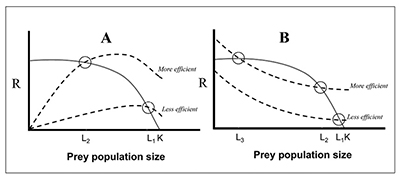
Figure 6. Examples of simplistic Lotka-Volterra type predator-prey models (Begon and Mortimer, 1981), showing prey growth rate (solid line) and predator total response curves (or per capita predation rate; dashed line) as a function of prey population size. The prey growth rate is maximum at low and mid prey densities, and declines to 0 at ecological carrying capacity (K). Where the two lines cross (Ls) are the equilibrium levels of the prey population as a result of predation. Note that the Ls are always lower than K. Thus, these models assume additive mortality. Graph A shows density-dependent responses by predators, where predation pressure increases as prey density increases. Graph B shows depensatory (i.e., inversely density-dependent) responses by predators, where predation intensity increases as prey density declines. Depensatory predation can destabilize systems and drive prey to very low densities and even extinction. In both cases, more efficient or multiple efficient predators are assumed to have a greater effect on prey numbers.
The degree of density dependence in predator populations can also cloud predator-prey models. For example, the numerical response of predators is naively assumed to increase as prey populations increase. However, many predators have density-dependent checks on population growth, which may include social regulation, territoriality, intolerance, stress, despotism, infanticide, or physiological density dependence as described above (e.g., Quigley and Hornocker, 2009; Wallach et al., 2015). These can cause populations of some predators to limit their population size because of social or other stress associated with encounters with conspecifics (Figure 7). Hence, predators might not be able to reach densities where they can limit healthy prey populations.
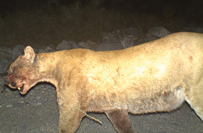
Figure 7. Life is no easier for the predator than for their prey. This puma likely had a territorial fight with another, and suffered some serious wounds as a result. Predator behaviors, such as territoriality, intolerance, despotism, and infanticide, can result in predator populations not being able to reach densities where they can limit healthy prey populations. (Photo courtesy of L. Bender.)
Last, population trend or trends in juvenile:female or other ratios by themselves cannot indicate the effect of predation because populations can be influenced concurrently by many factors, including predation, weather, habitat alterations, and density dependence, among others (Bender and Weisenberger, 2005, 2009; Christie et al., 2015; see 3. Confounded predator control examples, below). Many studies do not assess these other effects that can influence population trend when investigating predator-prey relationships (National Research Council, 1997; Mech, 2012). Relatedly, indirect effects of predation can potentially decrease prey productivity and population size by affecting prey foraging and distribution (Hernandez and Laundre 2005; Gude et al., 2006) even if the direct effect of predation has no impact on prey populations.
3. Confounded predator control examples.
For predator control programs to work, predation must be primarily additive on the prey population. If additive, then decreases in predators and thus predation should increase survival of prey. Successful predator control programs are hard to find outside of Alaska and situations involving introduced exotic predators, especially on islands (Jones et al., 2016). (Interestingly, this latter case is also true regarding many introductions of herbivores—a plant predator—onto islands where the prey—plants—are not adapted to herbivory [e.g., Klein, 1968].) Evidence supporting predator control in the Southwest is mostly inferred from historical retrospectives such as the history of mule deer on the Kaibab Plateau of Arizona (Heffelfinger, 2006). While increases in mule deer on the Kaibab are frequently attributed to predator removal, they were also influenced by extensive declines in the number of livestock, above-normal precipitation, eliminating female harvest, etc. (Mann and Locke, 1931; Heffelfinger, 2006). Which of these many factors contributed the most to increases is unknown.
Similarly, studies that show increased population-level recruitment or population size in large areas following predator control seldom account for other factors that could concurrently affect prey populations (e.g., pronghorn-coyote [Canis latrans]; Brown and Conover, 2011), such as drought, winter severity, and human alterations of the landscape (Christie et al., 2015). Hence, such correlative studies often yield conflicting results, e.g., coyote control favored pronghorn but not mule deer (Brown and Conover, 2011), or coyote control had no effect on pronghorn, whereas weather and landscape development did (Christie et al., 2015). Both results could well be correct for the given set of ecological conditions at each site. However, results from investigations such as these should be viewed with caution and not generalized beyond their study areas if they fail to account for other factors that may affect prey dynamics. Such investigations invariably fail to account for the complexities of predation.
Other manipulative or correlative tests have shown no effect from predator removals. For example, little evidence supports puma control having any effect on mule deer populations in the Southwest or elsewhere (Logan and Sweanor, 2001; Heffelfinger, 2006; Hurley et al., 2011; Forrester and Wittmer, 2013; Bender and Rosas-Rosas, 2016). To illustrate, in a seven-month period Logan and Sweanor (2001) removed 13 adult and subadult pumas from an estimated population of 16 on a treatment area within the San Andres Mountains. Survival of adult female mule deer did not differ prior to or after removals (Bender and Rosas-Rosas, 2016). Similar results were also seen in desert bighorn; ewe and ram survival did not differ when comparing the three years prior to (survival = 0.83) and the three years during and after (survival = 0.81) puma removals (Logan and Sweanor, 2001; Bender et al., 2017).
Conclusions
Predisposition is a prerequisite for compensatory mortality (Bender and Rosas-Rosas, 2016), so whenever any degree of predisposition is known or likely to be present, predation should not be assumed to limit prey even if it is the primary cause of death. Nor does low density of prey populations in the Southwest indicate that little density dependence is present in the prey, and therefore predation is likely to be additive because of a lack of density-dependent predisposition. Especially in the Southwest, conditions such as drought can reduce condition and predispose individuals to mortality regardless of the numbers present because forage quality or habitat cover may be inadequate regardless of population density (e.g., DeYoung et al., 2000; Ballard et al., 2003; Bender and Cook, 2005). Thus, for example, precipitation has consistently been shown to be the primary influence on ungulates in the Southwest (Smith and LeCount, 1979; Marshal et al., 2002; Bender and Weisenberger, 2005, 2009; DeVos and Miller, 2005; Brown et al., 2006; Heffelfinger, 2006; Simpson et al. 2007; Bender et al., 2007, 2011, 2012, 2013; McKinney et al., 2008), not predation (Heffelfinger, 2006; Bender and Rosas-Rosas, 2016; Bender et al., 2017).
This is not meant to imply that predation has no effect on wildlife in the Southwest. Given amendable circumstances, it certainly can and does. However, the common perception of a uniform deleterious effect is mistaken, and any effect, whether negative or none, is completely dependent upon the factors affecting the hierarchy of predation locally, particularly at the individual and population levels. Attempts to shortcut understanding of these local factors with simplistic metrics or additive models have driven the confusion and oversimplification of this complex ecological situation.
Acknowledgements
This project was funded by the private landowners of the Santa Fe Trail Adaptive Management Project, U.S. Department of Defense, U.S. Forest Service, U.S. Fish and Wildlife Service, U.S. Bureau of Land Management, New Mexico Department of Game and Fish, and New Mexico State University. The New Mexico Cooperative Extension Service provided additional financial support. I thank C. Allison, R. Baldwin, A. Darrow, T. Kavalok, and O. Rosas-Rosas for insightful critiques of this circular.
Literature Cited
Ballard, W.B., and V. Van Ballenberghe. 1998. Predator/prey relationships. In A.W. Franzmann and C.C. Schwartz (Eds.), Ecology and management of the North American moose (pp. 247–273). Washington, D.C.: Smithsonian Institute Press.
Ballard, W.B., D. Lutz, T.W. Keegan, L.H. Carpenter, and J.C. DeVos, Jr. 2003. Deer-predator relationships. In N.E. Headrick, M.R. Conover, and J.C. DeVos, Jr. (Eds.), Mule deer conservation: Issues and management challenges (pp. 177–218). Logan, UT: Jack H. Berryman Institute.
Bartmann, R.M., G.C. White, and L.H. Carpenter. 1992. Compensatory mortality in a Colorado mule deer population. Wildlife Monographs, 121, 1–39.
Begon, M., and M. Mortimer. 1981. Population ecology: A unified study of plants and animals. Sunderland, MA: Sinauer Associates.
Bender, L.C. 2008. Age structure and population dynamics. In S.E. Jorgensen and B.D. Fath (Eds.), Encyclopedia of ecology, 1st ed., vol. 1 (pp. 65–72). Oxford, UK: Elsevier B.V.
Bender, L.C. 2011. Basics of trophy management [Guide L-111]. Las Cruces: New Mexico State University Cooperative Extension Service. https://pubs.nmsu.edu/_l/L111/
Bender, L.C. 2013. Using population ratios for managing big game [Circular 669]. Las Cruces: New Mexico State University Cooperative Extension Service. https://pubs.nmsu.edu/_circulars/CR669/
Bender, L.C. 2018. Age structure and population dynamics [In press]. In B.D. Fath (Ed.), Encyclopedia of ecology, 2nd ed. Oxford, UK: Elsevier B.V.
Bender, L.C., and J.G. Cook. 2005. Nutritional condition of elk in Rocky Mountain National Park. Western North American Naturalist, 65, 329–334.
Bender, L.C., and B.D. Hoenes. 2017. Age-related fecundity of mule deer in south-central New Mexico. Mammalia [Online]. doi: https://doi.org/10.1515/mammalia-2016-0166
Bender, L.C., and O.C. Rosas-Rosas. 2016. Compensatory puma predation on adult female mule deer in New Mexico. Journal of Mammalogy, 97, 1399–1405.
Bender, L.C., and M. Weisenberger. 2005. Precipitation, density, and population dynamics of desert bighorn sheep on San Andres National Wildlife Refuge, New Mexico. Wildlife Society Bulletin, 33, 956–964.
Bender, L.C., and M.E. Weisenberger. 2009. Criticisms biologically unwarranted and analytically irrelevant: Reply to Rominger et al. Journal of Wildlife Management, 73, 806–810.
Bender, L.C., B.D. Hoenes, and C.L. Rodden. 2012. Factors influencing survival of desert mule deer in the greater San Andres Mountains, New Mexico. Human-Wildlife Interactions, 6, 245–260.
Bender, L.C., L.A. Lomas, and J. Browning. 2007. Condition, survival, and cause-specific mortality of adult female mule deer in north-central New Mexico. Journal of Wildlife Management, 71, 1118–1124.
Bender, L.C., O.C. Rosas-Rosas, and M.E. Weisenberger. 2017. Distribution, vulnerability, and predator-prey relationships of pumas and prey in the San Andres Mountains, south-central New Mexico. Final Report, San Andres National Wildlife Refuge, Las Cruces, New Mexico, USA.
Bender, L.C., J.C. Boren, H. Halbritter, and S. Cox. 2011. Condition, survival, and productivity of mule deer in semiarid grassland-woodland in east-central New Mexico. Human-Wildlife Interactions, 5, 276–286.
Bender, L.C., J.C. Boren, H. Halbritter, and S. Cox. 2013. Factors influencing survival and productivity of pronghorn in a semiarid grassland-woodland in east-central New Mexico. Human-Wildlife Interactions, 7, 313–324.
Bowyer, R.T., J.G. Kie, D.K. Person, and K.L. Monteith. 2013. Metrics of predation: Perils of predator-prey ratios. Acta Theriologica, 58, 329–340.
Boyce, M.S., A.R.E. Sinclair, and G.C. White. 1999. Seasonal compensation of predation and harvesting. OIKOS, 87, 419–426.
Brown, D.E., and M.R. Conover. 2011. Effects of large-scale removal of coyotes on pronghorn and mule deer productivity and abundance. Journal of Wildlife Management, 75, 876–882.
Brown, D.E., D. Warnecke, and T. McKinney. 2006. Effects of midsummer drought on mortality of doe pronghorn (Antilocapra americana). Southwestern Naturalist, 51, 220–225.
Caltrider, T., and L.C. Bender. 2017. Relationships between landscape greenness and condition of elk, mule deer, and pronghorn in New Mexico. Rangeland Ecology and Management [Online]. http://doi.org/10.1016/j.rama.2017.10.003
Christie, K.S., W.F. Jensen, J.H. Schmidt, and M.S. Boyce. 2015. Long-term changes in pronghorn abundance index linked to climate and oil development in North Dakota. Biological Conservation, 192, 445–453.
Cook, J.G. 2002. Nutrition and food. In D.E Toweill and J.W. Thomas (Eds.), North American elk: Ecology and management, 2nd ed. (pp. 259–349). Washington, D.C.: Smithsonian Institution Press.
Cook, J.G., B.K. Johnson, R.C. Cook, R.A. Riggs, T. Delcurto, L.D. Bryant, and L.L. Irwin. 2004. Effects of summer-autumn nutrition and parturition date on reproduction and survival of elk. Wildlife Monographs, 155, 1–61.
Cook, R.C., J.G. Cook, D.L. Murray, P. Zager, B.K. Johnson, and M.W. Gratson. 2001. Development of predictive models of nutritional condition for Rocky Mountain elk. Journal of Wildlife Management, 65, 973–987.
Dambacher, J.M., H.W. Li, J.O. Wolff, and P.A. Rossignol. 1999. Parsimonious interpretation of the impact of vegetation, food, and predation on snowshoe hare. OIKOS, 84, 530–532.
Depperschmidt, J.D, S.C. Torbit, A.W. Alldredge, and R.D. Deblinger. 1987. Body condition indices for starved pronghorns. Journal of Wildlife Management, 51, 675–678.
DeVos, J.C., Jr., and W.H. Miller. 2005. Habitat use and survival of Sonoran pronghorn in years with above-average rainfall. Wildlife Society Bulletin, 33, 35–42.
DeYoung, R.W., E.C. Hellgren, T.E. Fulbright, W.F. Robbins, Jr., and I.D. Humphreys. 2000. Modeling nutritional carrying capacity for translocated desert bighorn sheep in western Texas. Restoration Ecology, 8, 57–65.
Doherty, T.S., A.S. Glen, D.G. Nimmo, E.G. Ritchie, and C.R. Dickman. 2016. Invasive predators and global biodiversity loss. Proceedings of the National Academy of Sciences, 113, 11261–11265.
Errington, P.L. 1946. Predation and vertebrate populations. Quarterly Review of Biology, 21, 144–177, 221–245.
Errington, P.L. 1967. Of predation and life. Ames: Iowa State University Press.
Forrester, T.D., and H.U. Wittmer. 2013. A review of the population dynamics of mule deer and black-tailed deer Odocoileus hemionus in North America. Mammal Review, 43, 292–308.
Gaillard, J.-M., M. Festa-Bianchet, N.G. Yoccoz, A. Loison, and C. Toigo. 2000. Temporal variation in fitness components and population dynamics of large herbivores. Annual Review of Ecology and Systematics, 31, 367–393.
Gude, J.A., R.A. Garrott, J.J. Borkowski, and F. King. 2006. Prey risk allocation in a grazing ecosystem. Ecological Applications, 16, 285–298.
Hanks, J. 1981. Characterization of population condition. In C.W. Fowler and T.D. Smith (Eds.), Dynamics of large mammal populations (pp. 47–73). Caldwell, NJ: Blackburn Press.
Hassel, M.P. 1978. The dynamics of arthropod predator-prey systems. Princeton, NJ: Princeton University Press.
Heffelfinger, J. 2006. Deer of the Southwest: A complete guide to the natural history, biology, and management of Southwestern mule deer and white-tailed deer. College Station: Texas A&M University Press.
Hernandez, L., and J. Laundre. 2005. Foraging in the ‘landscape of fear’ and its implications for habitat use and diet quality of elk Cervus elaphus and bison Bison bison. Wildlife Biology, 11, 215–220.
Hoenes, B.D. 2008. Identification of factors limiting desert mule deer populations in the greater San Andres Mountains of southcentral New Mexico [Thesis]. Las Cruces: New Mexico State University.
Hornocker, M.G. 1970. An analysis of mountain lion predation upon mule deer and elk in the Idaho Primitive Area. Wildlife Monographs, 21, 1–39.
Hurley, M.A., J.W. Unsworth, P. Zager, M. Hebblewhite, E.O. Garton, D.M. Montgomery, J.R. Skalski, and C.L. Maycock. 2011. Demographic response of mule deer to experimental reduction of coyotes and mountain lions in southeastern Idaho. Wildlife Monographs, 178, 1–33.
Jones, H.P., and others. 2016. Invasive mammal eradication on islands results in substantial conservation gains. Proceedings of the National Academy of Sciences, 113, 4033–4038.
Klein, D.R. 1968. The introduction, increase, and crash of reindeer on St. Matthew Island. Journal of Wildlife Management, 32, 350–367.
Klein, D.R. 1981. The problem of overpopulation of deer in North America. In P.A. Jewell, S. Holt, and D. Hart (Eds.), Problems in the management of locally abundant wild mammals (pp. 119–127). New York: Academic Press.
Krausman, P.R., R. Valdez, and J.A. Bissonette. 1996. Bighorn sheep and livestock. In P.R. Krausman (Ed.), Rangeland wildlife (pp. 237–243). Denver, CO: Society for Range Management.
Krumm, C.E., M.M. Conner, and M.W. Miller. 2005. Relative vulnerability of chronic wasting disease infected mule deer to vehicle collisions. Journal of Wildlife Diseases, 41, 503–511.
Krumm, C.E., M.M. Conner, N.T. Hobbs, D.O. Hunter, and M.W. Miller. 2010. Mountain lions prey selectively on prion-infected mule deer. Biological Letters, 6, 209–211.
Kunkel, K., and D.H. Pletscher. 1999. Species-specific population dynamics of cervids in a multipredator ecosystem. Journal of Wildlife Management, 63, 1082–1093.
Logan, K.A., and L.L. Sweanor. 2001. Desert puma: Evolutionary ecology and conservation of an enduring carnivore. Washington, D.C.: Island Press.
Lomas, L.A., and L.C. Bender. 2007. Survival and cause-specific mortality of neonatal mule deer fawns, north-central New Mexico. Journal of Wildlife Management, 71, 884–894.
Mann, W.G., and S.B. Locke. 1931. The Kaibab deer: A brief history and recent developments [Unpublished report]. Fredonia, AZ: U.S. Forest Service, Kaibab National Forest.
Marshal, J.P., P.R. Krausman, V.C. Bleich, W.B. Ballard, and J.S. McKeever. 2002. Rainfall, El Niño, and dynamics of mule deer in the Sonoran Desert, California. Journal of Wildlife Management, 66, 1283–1289.
McKinney, T., D.E. Brown, and L. Allison. 2008. Winter precipitation and recruitment of pronghorns in Arizona. Southwestern Naturalist, 53, 319–325.
Mech, L.D. 2012. Is science in danger of sanctifying the wolf? Biological Conservation, 150, 143–149.
Mech, L.D., and R.O. Peterson. 2003. Wolf-prey relations. In L.D. Mech and L. Boitani (Eds.), Wolves: Behavior, ecology, and conservation (pp. 131–160). Chicago, IL: University of Chicago Press.
National Research Council. 1997. Wolves, bears, and their prey in Alaska: Biological and social challenges in wildlife management. Washington, D.C.: National Academy Press.
National Research Council. 2002. Ecological dynamics on Yellowstone’s northern range. Washington, D.C.: National Academy Press.
Okarma, H. 1991. Marrow fat content, sex and age of red deer killed by wolves in winter in the Carpathian Mountains. Holarctic Ecology, 14, 169–172.
Phillips, G.E., and A.W. Alldredge. 2000. Reproductive success of elk following disturbance by humans during calving season. Journal of Wildlife Management, 64, 521–530.
Polisar, J., I. Maxit, D. Sconagmillo, L. Farrel, M.E. Sunquist, and J.F. Eisenberg. 2003. Jaguars, pumas, their prey base, and cattle ranching: Ecological interpretation of a management problem. Biological Conservation, 109, 297–310.
Quigley, H., and M. Hornocker. 2009. Cougar population dynamics. In M. Hornocker and S. Negri (Eds.), Cougar: Ecology and conservation (pp. 59–75). Chicago, IL: University of Chicago Press.
Ratcliffe, P.R. 1980. Bone marrow fat as an indicator of condition in roe deer. Acta Theriologica, 25, 26, 333–340.
Rosas-Rosas, O.C., L.C. Bender, and R. Valdez. 2008. Jaguar and puma predation on cattle calves in northeastern Sonora, Mexico. Rangeland Ecology and Management, 61, 554–560.
Rosas-Rosas, O.C., L.C. Bender, and R. Valdez. 2010. Habitat correlates of jaguar kill-sites of cattle in northeastern Sonora, Mexico. Human-Wildlife Interactions, 4, 113–121.
Ruth, T.K., and K. Murphy. 2009. Cougar-prey relationships. In M. Hornocker and S. Negri (Eds.), Cougar: Ecology and conservation (pp. 138–172). Chicago, IL: University of Chicago Press.
Simpson, D.C., L.A. Harveson, C.E. Brewer, R.A. Walser, and A.R. Sides. 2007. Influence of precipitation on pronghorn demography in Texas. Journal of Wildlife Management, 71, 906–910.
Sinclair, A.R.E. 2003. Mammal population regulation, keystone processes and ecosystem dynamics. Philosophical Transactions of the Royal Society of London B, 358, 1729–1740.
Sinclair, A.R.E., and R.P. Pech. 1996. Density dependence, stochasticity, compensation and predator regulation. OIKOS, 75, 164–173.
Smith, R.H., and A. Lecount. 1979. Some factors affecting survival of desert mule deer fawns. Journal of Wildlife Management, 43, 657–665.
Theberge, J.R. 1990. Potentials for misinterpreting impacts of wolf predation through predator:prey ratios. Wildlife Society Bulletin, 18, 188–192.
Wakeling, B.F., and L.C. Bender. 2003. Influence of nutrition on mule deer biology and ecology. In J.C. deVos, Jr., M. Conover, and N. Headrick (Eds.), Mule deer conservation: Issues and management strategies (pp. 93–116). Logan, UT: Jack Berryman Institute Press.
Wallach, A.D., I. Izhaki, J.D. Toms, W.J. Ripple, and U. Shanas. 2015. What is an apex predator? OIKOS, 124, 1453–1461.
Wilmers, C.C., E. Post, and A. Hastings. 2007. The anatomy of predator-prey dynamics in a changing climate. Journal of Animal Ecology, 76, 1037–1044.
For further reading
CR-662: Guidelines for Management of Habitat for Mule Deer
https://pubs.nmsu.edu/_circulars/CR662/
CR-664: Guidelines for Monitoring Elk and Mule Deer Numbers in New Mexico
https://pubs.nmsu.edu/_circulars/CR664/
CR-669: Using Population Rations for Managing Big Game
https://pubs.nmsu.edu/_circulars/CR669/

Lou Bender is a Research Scientist (Wildlife) with the Department of Extension Animal Sciences and Natural Resources at NMSU. He earned his Ph.D. from Michigan State University. His research and management programs emphasize ungulate and carnivore management, integrated wildlife and livestock habitat management, and wildlife enterprises in the Southwest and internationally.
To find more resources for your business, home, or family, visit the College of Agricultural, Consumer and Environmental Sciences on the World Wide Web at pubs.nmsu.edu
Contents of publications may be freely reproduced for educational purposes. All other rights reserved. For permission to use publications for other purposes, contact pubs@nmsu.edu or the authors listed on the publication.
New Mexico State University is an equal opportunity/affirmative action employer and educator. NMSU and the U.S. Department of Agriculture cooperating.
January 2018 Las Cruces, NM