Circular 669

Louis C. Bender

College of Agricultural, Consumer and Environmental Sciences, New Mexico State University

Senior Research Scientist (Natural Resources), Department of Extension Animal Sciences and Natural Resources, New Mexico State University. (Print Friendly PDF)

Introduction

Wildlife (hunting) enterprises are important sources of revenue for property owners in New Mexico. Elk (Cervus elaphus), mule deer (Odocoileus hemionus), and pronghorn (Antilocapra americana) are the main wildlife resources of most private landowners in New Mexico. Managing these game species requires monitoring and interpreting key population parameters to optimize harvest and trophy quality. Whether managing for maximum sustainable yield or trophy production, managers need to carefully monitor key demographics of their populations, most importantly productivity ratio (fawn:doe or calf:cow), adult sex ratio (bull:cow or buck:doe), and age structure. These provide the needed information to determine optimal harvest levels, which, combined with good nutrition, determine whether individuals can maximize their potential for reproduction (Bender et al., 2011, 2012b, 2013b; Halbritter and Bender, 2011b), antler size, or other animal quality measures (Bender, 2018a).

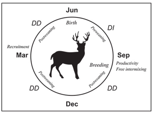
Figure 1. The biological year of most big game species in the western United States. Timing of key processes (e.g., periods of density-dependent [DD] and density-independent [DI] mortality, breeding seasons, etc.) must be incorporated into management surveys if survey data are to be relatively unbiased.

Productivity and Morality Rates

Determining sustainable or optimal harvests to achieve big game management goals is the key to effectively managing wildlife enterprises (Bender, 2018a). While trends in population size (Bender, 2012b, 2020) are useful for management, they alone do not provide the specific demographic data needed to determine optimal harvests of big game populations. Determining harvests requires information on production and mortality of populations, both of which can be determined from simple population ratios (Bender, 2006). These ratios include adult sex ratios (ASR), productivity or recruitment ratios, and age ratios, especially yearling percentages (% yearling). These ratios allow managers to determine (1) the maximum sustainable mortality rates for a population and (2) the current annual mortality rates, which are the key demographics used to effectively harvest populations and manipulate population structure. As with all management data, however, these ratios need to be collected during biologically meaningful periods and interpreted correctly.

The biological year for big game can be categorized into appropriate critical periods (Gaillard et al., 2000). These include birth, preweaning, and postweaning periods for juveniles, and the same periods plus the breeding season for adults (Figure 1). The breeding season is important because it represents the time when adults, especially adult males, are most likely to be freely intermixed with females and juveniles, and thus it is possible to collect relatively unbiased adult sex ratio information from the population (Figure 2). Moreover, if age classes are distinguishable by physical appearance, relatively unbiased population age structure can also be determined during periods of free intermixing.

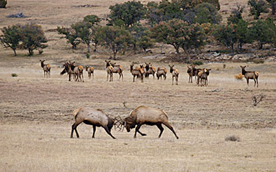
Figure 2. All herd components (males, females, juveniles) are as freely intermixed as they get during the breeding seasons. During this time, relatively unbiased productivity and adult sex ratio data can be collected. (Photo courtesy of M. Reardon/A. Darrow.)

The preweaning and postweaning periods are important because of changes in visibility of juveniles and in mortality patterns of juveniles and adults (Figure 3). Prior to weaning, observed juvenile:female (J:F) ratios tend to vary wildly, although they generally increase as juveniles progressively accompany their mothers as they get older (Progulske and Duerre, 1964; Geist, 1981; McCullough et al., 1994). Because juveniles are not reliably seen with adults during the preweaning period, J:F ratios collected in this period potentially have great bias and little management significance.

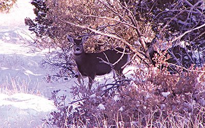
Figure 3. Fawns progressively accompany their mother as weaning progresses. Following weaning, juveniles are often freely intermixed with adult females. Consequently, relatively unbiased productivity and recruitment ratios can be collected from approximately weaning through age 1 to 1.5. (Photo courtesy of M. Reardon/A. Darrow.)

Additionally, causes of mortality of juveniles (and adults) during this late spring and summer period tend to be density independent, meaning that they are not related to competition for resources (food, water, cover, etc.). This is because food is annually most abundant during this period; there is little competition among adults, and juveniles are mostly dependent on their mothers for nutrition early in lactation. Hence, most losses are due to causes that managers cannot control (weather, accidents) and thus cannot effectively manage. The exception is that survival of juveniles is strongly related to maternal quality, and maternal investment can be enhanced by providing the best possible foraging conditions. Thus, although a logical goal of managers would be to maximize the numbers of juveniles that survive to weaning, the reality is that much of what most commonly causes losses of juveniles cannot be mitigated by management. Hence, even if J:F ratios were unbiased during this period, they would be of less interest to managers because their actions could only marginally influence this ratio during this time period. Despite this, it is always a good strategy to maximize the quality of big game habitat in order to produce and recruit as many juveniles as possible (Bender, 2012a, 2018a, 2019).

However, as weaning approaches, juveniles habitually travel with adult females, resulting in unbiased J:F ratios. Thus, weaning results in free intermixing of juveniles and adults, so ratios collected during this autumn period (hereafter referred to as productivity ratios) provide useful management data. Early autumn also coincides with the beginning of hunting for most big game in the Southwest, and data from harvested animals is often used by state agencies to estimate the immediate pre-hunting composition of the population (Burgoyne, 1981; Roseberry and Woolf, 1991; Bender and Spencer, 1999). The number of big game animals harvested on any single ranch is almost certainly too low for this approach, however, so landowners should use actual surveys to determine their population structure.

Following weaning, causes of mortality for both juveniles and adults tend to become increasingly density dependent as quantity and especially quality of food decline throughout the autumn. Density dependence in a population relates to factors that affect individual resource capture, such as competitive ability, herd numbers, quantity of forage, etc. These are all readily and commonly managed for (e.g., Bender, 2012a, 2018a, 2018b; Bender et al., 2012a, 2013b; Halbritter and Bender, 2011a), and both game and livestock managers try to avoid overpopulation or exceeding the carrying or range capacity of their lands specifically to avoid seeing density-dependent effects in their herds (i.e., for wildlife: low body mass, poor trophy quality, lower pregnancy rates, etc; for livestock: lower meat or fiber yields, lower milk output, lower pregnancy rates, etc.) (Bender, 2018a, 2019). Again, density-dependent factors can usually be directly managed for, allowing managers to maximize postweaning survival. While some events, such as extremely harsh winters or droughts, are difficult to manage for, the effects of events like these can be minimized by proper management and planning (Bender, 2012a; Bender et al., 2013a, 2013b).

The postweaning period ends with the recruitment of 1-year-olds into the adult age classes, where they typically become vulnerable to harvest. Ideally, recruitment ratios would be collected concurrently with productivity ratios in early autumn, but the difficulty in differentiating yearling age classes in females and the tendency for young males to disperse prior to or during the rut generally preclude collecting yearling:female ratios during this period. However, because density-independent mortality during the summer tends to be trivial for non-neonates (Gaillard et al., 2000), late spring J:F ratios (hereafter referred to as recruitment ratios) are generally an accurate indicator of true recruitment into the adult population (the age 1.5 and older hunting year class). It is important to collect recruitment ratio data in early spring, not in mid- or late winter, because potentially significant juvenile mortality associated with late winter and the winter-spring transition may be missed (Bender et al., 2013a).

Productivity Ratios

Productivity (preseason or autumn J:F) ratios can be used to determine the maximum sustainable mortality rates for the surveyed population. Because ratios for ungulates are expressed per 100 adult females, data can be interpreted as percentages and used to calculate the maximum mortality a population can withstand without declining.

Example: If a preseason survey of an elk population finds a J:F ratio of 40 calves/100 cows, and managers assume a juvenile sex ratio of 1:1, there are 20 female calves/100 cows. From this, the maximum sustainable mortality rate or the potential population yield (Y) for adult cows (Y_F) in this population is 20/100 = 20%, because there are a maximum of 20 new females available to replace the loss of 20 existing cows.

Similarly, if the adult sex ratio is known (or can be calculated; see Adult Sex Ratios section), then maximum sustainable mortality rates for males (Y_M) can also be determined. Continuing this example, if the bull/cow ratio in the surveyed population was 25/100, then there are a maximum of 20 juvenile bulls available to replace 20 adult bulls, for a Y_M of 20/25 = 0.80 or 80%. This rate can also be determined from Y_F and the inverse of the ASR; 0.20 × (100/25) = 0.80.

Note that this example assumes that all approximately 3- to 4-month-old juveniles survive until recruitment into the adult segment at age 1.5, which is unlikely (mean postweaning survival is 0.71 [SE = 0.03] for cervids and 0.68 [SE = 0.05] for bovids; Gaillard et al., 2000). This assumption can be addressed in two ways. First, survival can be assumed to be some constant proportion, such as the values from Gaillard et al. (2000). This approach has problems, though, because while postweaning survival is usually more consistent than preweaning, severe winters or droughts can decimate entire calf or fawn cohorts, resulting in no recruitment the following year. Thus, a better alternative is to estimate overwinter survival from either telemetry studies or from changes in ratios (i.e., Bender et al., 2002). For the latter, spring survey data are used to determine overwinter juvenile survival (S_J) from autumn survey data:

S_J = (spring J:F) / (autumn J:F)

Continuing with the example, if herd composition counts the following spring determined that recruitment ratios were 30 calves/100 cows, then S_J = 30/40 = 0.75. Note that this estimate of overwinter survival is a minimum estimate because the denominator in the ratios has likely changed (i.e., some adult females have died; Bender and Hall, 2004). Because the frame of reference of the ratio is the 100 cows in the autumn population, this means that the 30 calves/100 cows in the spring counts are actually 30 calves/<100 cows. The effect of this bias is to underestimate calf survival; thus, it introduces a measure of conservatism into management decisions based on these survival rates. Note, however, that if sample sizes are small or adult female harvest is very high, the spring ratio may not be truly representative of the population and can occasionally be larger than the autumn ratio. In these cases, the spring ratio is biased high and the autumn ratio should be used for management decisions because there likely was not significant overwinter mortality of juveniles.

Because of overwinter mortality of juveniles, for the previous example, maximum sustainable Y_F is reduced to 0.15 because of the 20 juvenile females available to replace the adults of the fall population, only 15 survived the winter (20 × 0.75 = 15). Similarly for the males, the maximum sustainable Y_M is decreased from 0.80 to 0.60 (i.e., [20 × 0.75]/25 = 0.60).

Finally, remember that these examples outline how to determine the maximum sustainable mortality rates, most of which managers can usually capture in harvest—but not all. Some mortality, usually <0.10 for females and <0.15 for males, will always occur due to old age, accidents, etc. For example, if a cow elk can live to about age 25 in the wild, about 1/25 or 4% of the population will be turned over annually due to senescence alone. Thus, there will always be at least a background mortality rate of 0.04 that managers need to subtract from their maximum sustainable rates when estimating their harvestable surplus (unless the goal is to decrease the population by harvesting above sustainable yield). Further, maximum sustainable rates may not be the optimal rates; for example, if managing for trophy production, maximum sustainable rates for adult males will certainly be much higher than the rate needed to allow survival into older age classes (see Mortality Rates section; Bender, 2018a, 2019). Optimal mortality rates need to be determined based on all management objectives, such as a desired bull:cow or buck:doe ratio or male age structure (Bender, 2018a).

Recruitment Ratios

Recruitment ratios alone can provide data on sustainable mortality rates if collected during biologically appropriate times (i.e., during the change from density-dependent to density-independent mortality patterns; Figure 1). As in the determination of overwinter juvenile survival, because the denominator of the source population has changed, spring recruitment ratios are a minimum indication of recruitment into the previous fall population. Use of these ratios to determine Y_F or Y_M is as described for productivity (autumn) ratios, with the exception that survival does not have to be incorporated.

Ideally, 1.5-year-old individuals would be sufficiently different from older adults to determine actual recruitment rates during productivity surveys (Smith and McDonald, 2002). For most North American ungulates, however, females are difficult to differentiate during this time, especially from aerial surveys, and numbers of 1.5-year-old males are as much a function of dispersal and immigration as of recruitment of the base population. However, the proportions of 1.5-year-olds is indicative of population-level recruitment for the study population (Burgoyne, 1981; Bender and Spencer, 1999), and thus can be used to determine actual mortality rates experienced by the adult segment of the population given certain assumptions (see Mortality Rates section).

Age Structure

Mortality Rates

Ratio data can also be used to determine the actual mortality rates experienced by populations (Bender, 2006). In an age-stable, stationary population where recruitment is defined as occurring at age 1.5, the percentage of yearling males in the prehunting male population equals the annual adult (age >1.5) male mortality rate (Burgoyne, 1981; Roseberry and Woolf, 1991). This mortality rate also is equivalent to the grand mean of all age-specific mortality rates, weighted by numbers in each age class, from a life table analysis (Bender and Spencer, 1999). What this means is fairly simple: Picture a full glass of water; this is the age-stable, stationary population. If 10 ounces of water are added to the full glass, 10 ounces must flow out. The added 10 ounces is the recruitment, and the lost 10 ounces is the mortality. If the glass holds 20 ounces, then the recruitment (yearling percentage) and mortality rate both equal 10/20, or 0.50.

This approach assumes that the population is age-stable and stationary, meaning that its size is neither increasing nor declining (stationary) and that the relative proportions of individuals in each age class do not change (age-stable). Neither of these assumptions is likely to be met in free-ranging populations. Hence, the yearling percentage will slightly overestimate the true mortality rate if the population is increasing (because proportionally more yearlings are entering the adult male population; i.e., age structure is declining), and will slightly underestimate the true mortality rate if the population is declining (because fewer young are being produced and hence proportionally fewer yearling males are being recruited relative to past years; Roseberry and Woolf, 1991). Mortality rates can be corrected for population trend, but the correction is usually small (Bender, 2006) and unlikely to affect interpretations for most managers. See Bender (2006) for directions on how to correct mortality rates for population trend, if desired.

Example: If an autumn composition survey indicated that there were 25 males/100 females, and that 20 of those males were subjectively classified as yearlings (typically by antler characteristics), then:

Male mortality rate = M_M = 20/25 = 0.80

For females and species that cannot be aged from aerial surveys, age structure of harvested animals can be used to determine the yearling proportions if harvest can be assumed to be reasonably unselective of age class and harvests are large; this approach is often used by state agencies at the game management unit level or larger. The more intensively hunted a population is, the more likely this assumption is to be true. Bender and Spencer (1999) and Bender et al. (2004) corroborated the use of yearling proportions for estimating mortality rates of male elk and black-tailed deer (O. hemionus columbianus), respectively, over a variety of harvest intensities. As a note of caution, managers should be aware of the nutritional status of their herds when classifying males into yearling or older age classes. The better the nutrition, the better the antler development of yearlings can be (Bender, 2018a) and the more difficult it becomes to classify yearlings based solely on antler characteristics.

Once estimated, managers can increase or decrease male harvest to meet their management goals. Most commonly, private land managers will manage for trophy production, which requires survivorship into older age classes (Bender, 2018a). Allowing males to survive into older age classes in turn requires very low adult male mortality rates (Figure 4), much lower than the maximum sustainable levels (Bender, 2018a, 2019). Alternatively, if the management goal was to harvest as many bucks or bulls as possible and the estimated annual mortality rate (from age structure) is lower than the maximum sustainable mortality rate (from productivity data), harvest can be increased incrementally until these rates approximately align.

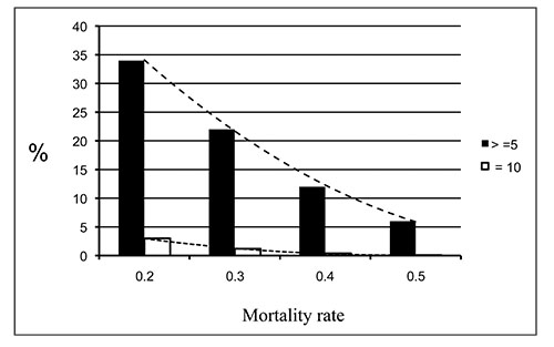
Figure 4. Effects of increasing adult male mortality rate on survivorship of adult males into ages >5 or age 10. With a 20% mortality rate, about 34% of males live to age 5 and older, and about 3% reach age 10. If mortality rates are increased to 50%, only 6% of the population will live to age 5 or older, and <0.1% will reach age 10. Average productivity can often support sustainable yields of >50%, but trophy production requires much lower mortality rates, usually <30%.

Adult Sex Ratios

For ranch managers, ASRs should be directly determined from relatively unbiased preseason composition surveys. Occasionally, state agencies estimate ASRs directly from mortality rates (i.e., ASR = M_F/M_M; Lang and Wood, 1976), derived from population age structure data collected from hunter check stations (Lang and Wood, 1976). This latter approach does highlight a key element that managers need to understand: ASRs do not occur by chance in a population, nor are they solely the product of male harvest rate. Rather, they integrate both male and female mortality rates. For example:

If M_F = 0.20 and M_M = 0.80, then

ASR = M_F/M_M = 0.20/0.80 = 0.25
= 25 males/100 females

Remember, ASRs are due to the interaction of M_F and M_M rates, not solely due to M_M. Thus, any change in either male or female mortality rates will affect the ASR. In general, as male mortality goes down, buck:doe or bull:cow ratios increase. Thus, ASR is often (mistakenly) used as a surrogate for male mortality rate. However, that is only partially true. Actually measuring male mortality is far more accurate than using ASR as a surrogate and requires the same data. Because managing for maximum sustainable yields (see PRODUCTIVITY RATIOS section) or trophy management (Bender, 2018a) both require careful monitoring of male mortality rate, managers should use mortality rate estimates derived from relatively unbiased surveys—not surrogates—for optimal management of their big game populations.

Collecting Composition Data

The same unbiased composition data can be used to determine how much mortality—including harvest—a population can withstand without declining and what the mortality rate of the population was for the prior year. In short, everything a manager needs to know for optimal harvesting comes from the collection of simple, unbiased composition data. The best way to collect this data is from helicopter surveys; similar data can be collected from ground surveys, but the ASR and age structure data may not be as accurate (Bender et al., 2003). Preliminary data from an ongoing multiyear study of mine on a northern New Mexico ranch also suggests that a well-designed camera-trap grid can produce data similar to ground (and possibly aerial) surveys.

Further, the optimal time for surveys is during, or just after, the breeding season, so it differs for most big game species in New Mexico. Timing for unbiased surveys of elk and pronghorn would be in late September or early October, although pronghorn, because segregation of the sexes is minimal, can usually be adequately surveyed any time during autumn (Figure 5). Mule deer surveys are best accomplished late, usually in December. Because many hunting seasons are over by this time, unbiased preseason composition can be estimated by adding the harvested bucks into your December survey totals if the number harvested is large enough to affect the ratio (Bender, 2012b).

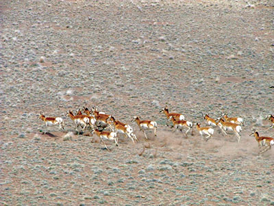
Figure 5. Pronghorn can be successfully surveyed and sex and age ratios can be gathered throughout much of the year, but the males are most likely to be with female groups during early autumn (September). (Photo courtesy of E. Watters.)

Acknowledgments

I thank R. Baldwin, J. Boren, A. Darrow, B. Hoenes, and T. Kavalok for constructive reviews of this circular. Funding was provided by New Mexico State University’s Agricultural Experiment Station, Cooperative Extension Service, and Corona Range and Livestock Research Center; the Santa Fe Trail Mule Deer Adaptive Management Project (STAMP); the New Mexico Department of Game and Fish; the Rocky Mountain Elk Foundation; and multiple private landowners throughout New Mexico.

Literature Cited

Bender, L.C. 2006. Uses of herd composition ratios in ungulate management. Wildlife Society Bulletin, 34, 1225–1230.

Bender, L.C. 2012a. Habitat management guidelines for mule deer: Piñon-juniper, Chihuahuan desert, arid grasslands, and associated arid habitat types [Circular 662]. Las Cruces: New Mexico State University Cooperative Extension Service.

Bender, L.C. 2012b. Guidelines for monitoring elk and mule deer numbers in New Mexico [Circular 664]. Las Cruces: New Mexico State University Cooperative Extension Service.

Bender, L.C. 2018a. Basics of trophy management [Guide L-111]. Las Cruces: New Mexico State University Cooperative Extension Service.

Bender, L.C. 2018b. Burning for big game [Circular 657]. Las Cruces: New Mexico State University Cooperative Extension Service.

Bender, L.C. 2019. Age structure and population dynamics. In B.D. Fath (Ed.), Encyclopedia of ecology, 2nd ed., vol. 1 (pp. 135–143). Oxford, UK: Elsevier B.V.

Bender, L.C. 2020. Guidelines for monitoring big game populations in New Mexico II: Trend indices in press. Las Cruces: New Mexico State University Coop­erative Extension Service.

Bender, L.C., and R. Spencer. 1999. Estimating elk population size by reconstruction from harvest data and herd ratios. Wildlife Society Bulletin, 27, 636–645.

Bender, L.C., and P.B. Hall. 2004. Winter survival in black-tailed deer populations affected by hair-loss syndrome. Journal of Wildlife Diseases, 40, 444–451.

Bender, L.C., W.L. Myers, and W.R. Gould. 2003. A comparison of ground and helicopter counts for determining North American elk Cervus elaphus and mule deer Odocoileus hemionus population composition. Wildlife Biology, 9, 199–205.

Bender, L.C., R.A. Baldwin, and J.R. Piasecke. 2012a. Multiscale habitat associations and habitat-condition relationships of elk in desert grassland-scrubland, northwestern New Mexico. Southwestern Naturalist, 57, 361–369.

Bender, L.C., B.D. Hoenes, and C.L. Rodden. 2012b. Factors influencing survival of desert mule deer in the greater San Andres Mountains, New Mexico. Human-Wildlife Interactions, 6, 245–260.

Bender, L.C., E. Carlson, S.M. Schmitt, and J.B. Haufler. 2002. Production and survival of elk (Cervus elaphus) calves in Michigan. American Midland Naturalist, 148, 163–171.

Bender, L.C., J.C. Boren, H. Halbritter, and S. Cox. 2011. Condition, survival, and productivity of mule deer in semiarid grassland-woodland in east-central New Mexico. Human-Wildlife Interactions, 5, 276–286.

Bender, L.C., J.C. Boren, H. Halbritter, and S. Cox. 2013a. Factors influencing survival and productivity of pronghorn in a semiarid grassland-woodland in east-central New Mexico. Human-Wildlife Interactions, 7, 313–324.

Bender, L.C., J.C. Boren, H. Halbritter, and S. Cox. 2013b. Effects of site characteristics, pinyon-juniper control, and precipitation on habitat quality for mule deer in New Mexico. Human-Wildlife Interactions, 7, 47–59.

Bender, L.C., G.A. Schirato, R.D. Spencer, K.R. McAllister, and B.L. Murphie. 2004. Survival, cause-specific mortality, and harvesting of buck black-tailed deer in Washington. Journal of Wildlife Management, 68, 870–878.

Burgoyne, Jr., G.E. 1981. Observations on a heavily exploited deer population. In C.W. Fowler and T.D. Smith (Eds.), Dynamics of large mammal populations (pp. 403–413). New York: John Wiley and Sons.

Gaillard, J.-M., M. Festa-Bianchet, N.G. Yoccoz, A. Loison, and C. Toigo. 2000. Temporal variation in fitness components and population dynamics of large herbivores. Annual Review of Ecology and Systematics, 31, 367–393.

Geist, V. 1981. Behavior: Adaptive strategies in mule deer. In O.C. Wallmo (Ed.), Mule and black-tailed deer of North America (pp. 157–224). Lincoln: University of Nebraska Press.

Halbritter, H., and L.C. Bender. 2011a. Elk habitat quality in the southern Sacramento Mountains, New Mexico. Southwestern Naturalist, 56, 1–8.

Halbritter, H., and L.C. Bender. 2011b. Condition, survival, and productivity of elk in the Sacramento Mountains of southern New Mexico. Southwestern Naturalist, 56, 305–314.

Lang, L.M., and G.W. Wood. 1976. Manipulation of the Pennsylvania deer herd. Wildlife Society Bulletin, 4, 159–166.

McCullough, D.R., F.W. Weckerly, P.I. Garcia, and R.R. Evett. 1994. Sources of inaccuracy in black-tailed deer herd composition counts. Journal of Wildlife Management, 58, 319–329.

Progulske, D.R., and D.C. Duerre. 1964. Factors influencing spotlight counts of deer. Journal of Wildlife Management, 28, 27–34.

Roseberry, J.L., and A. Woolf. 1991. A comparative evaluation of techniques for analyzing white-tailed deer harvest data. Wildlife Monographs, 117, 1–59.

Smith, B.L., and T.L. McDonald. 2002. Criteria to improve age classification of antlerless elk. Wildlife Society Bulletin, 30, 200–207.

For Further Reading

CR-605: Establishing a Shooting Preserve as a Means of Diversification for Landowners in New Mexico
pubs.nmsu.edu/_circulars/CR605/

CR-662: Guidelines for Management of Habitat for Mule Deer: Piñon-juniper, Chihuahuan desert, arid grasslands, and associated arid habitat types
pubs.nmsu.edu/_circulars/CR662/

CR-664: Guidelines for Monitoring Elk and Mule Deer Numbers in New Mexico
pubs.nmsu.edu/_circulars/CR664/

To find more resources for your business, home, or family, visit the College of Agricultural, Consumer and Environmental Sciences on the World Wide Web at pubs.nmsu.edu.

Contents of publications may be freely reproduced, with an appropriate citation, for educational purposes. All other rights reserved. For permission to use publications for other purposes, contact pubs@nmsu.edu or the authors listed on the publication.

New Mexico State University is an equal opportunity/affirmative action employer and educator. NMSU and the U.S. Department of Agriculture cooperating.

Revised September 2020 Las Cruces, NM