Circular 664

Louis C. Bender

College of Agricultural, Consumer and Environmental Sciences, New Mexico State University

Senior Research Scientist (Natural Resources), Department of Extension Animal Sciences and Natural Resources, New Mexico State University. (Print Friendly PDF)

Introduction

Wildlife (hunting) enterprises are important sources of revenue for property owners in New Mexico, and consequently elk (Cervus elaphus) and mule deer (Odocoileus hemionus) are vital economic resources for private landowners (Figure 1). Sustainable management of these resources requires monitoring of populations. This is particularly true in arid habitats where annual changes in population productivity, and thus sustainable harvest and trophy quality, can be pronounced (Heffelfinger et al., 2003; Bender, 2011).

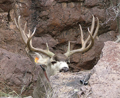
Figure 1. Wildlife such as mule deer can contribute significantly to ranch income through well-managed wildlife hunting enterprises. Managing populations for optimal yields requires accurate monitoring of population size and composition. (Photo courtesy of E. Watters.)

Many methods have been used to monitor the status, composition, and trends of deer and elk populations. Methods range from trend indices (Bender, 2020a), which provide information on whether a population is increasing, stable, or declining, to abundance estimators, which provide a population estimate (Lancia et al., 1996). Population estimates are preferable to trend estimators for several reasons. First, they allow direct calculation of harvestable surplus. Second, population estimates can be converted to densities, and relationships between resource availability (forage, etc.) and population size can be determined. Ultimately, it is the per capita resource (food, water) availability that determines individual body condition and thus population productivity, harvestable surplus, and animal (trophy) quality (Bender, 2011).

The most common trend indices used by landowners include minimum counts, spotlight or ground counts, and pellet group surveys (Bender, 2020a). Unfortunately, most of these commonly used trend indices have many assumptions that usually result in trend information of uncertain value, and very few have been calibrated to actual population size (Keegan et al., 2011; Bender, 2020a). Consequently, these methods are seldom used by management agencies to monitor populations because of the inherent problems and inaccuracies in these methods.

Similarly, many methods are used to estimate the size of big game populations, including distance sampling, mark-resight estimators, and sight-bias or sightability models (Keegan et al., 2011). The most commonly used and probably best method is an aerial sight-bias (sightability) model (Samuel et al., 1987; Otten et al., 1993). Sightability model surveys can be expensive to conduct because they require the use of a helicopter (Figure 2), but they probably produce the best data for management of deer and elk populations and are the least complicated population estimator to use on wildlife enterprises. Thus, sightability models are the most useful and easily applied of the accurate methods for monitoring population size, and should be the tool of choice for landowners in New Mexico and similar habitats.

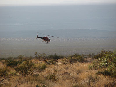
Figure 2. Using a helicopter provides many advantages for wildlife surveys. Herding individuals, viewing from many different angles, and low flight capability all greatly increase the accuracy of herd composition counts. (Photo courtesy of M. Weisenberger.)

Sightability Models

Sightability models estimate population size by correcting the number of observed elk or deer groups by the numbers missed due to incomplete detection. Detection is never complete because some animals are obscured by shadow, in vegetation, or otherwise hidden from view (Figure 3), and are thus missed during survey flights (Samuel et al., 1987). Many factors have been shown to affect detectability (Figures 4A and 4B), most commonly group size, activity (whether individuals are bedded, standing, or moving), amount and type of vegetative cover, topography, and presence or absence of snow cover (Caughley, 1974; Otten et al., 1993; Unsworth et al., 1994; Anderson et al., 1998; Cogan and Diefenbach, 1998). Sightability models develop correction factors for variables that significantly influence detectability for a particular species in a particular habitat (Samuel et al., 1987; Unsworth et al., 1994).

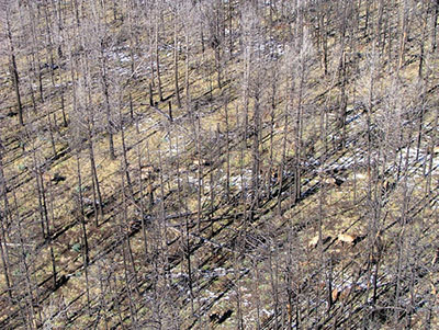
Figure 3. Individuals in groups are often not seen during surveys for a variety of reasons, including some individuals in a group being obscured by topography, vegetation, etc. Sightability models correct groups of elk or deer seen during surveys for groups missed using the group characteristics most important to detection. For both elk and mule deer, detection is primarily driven by the size of the group. However, even large groups can have individuals missed. For elk, the likelihood of seeing all individuals reaches approximately 100% at a group size of 19, much larger than most people would predict. (Photo courtesy of E. Watters.)

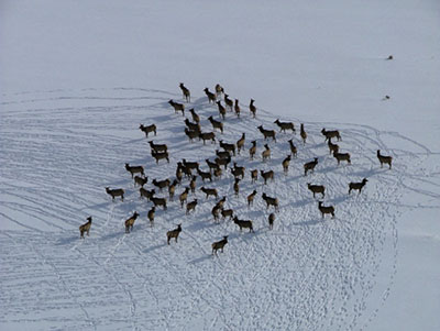
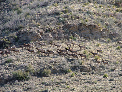
Figures 4A (top) and 4B (bottom). Many variables can potentially influence the likelihood of detecting a group of animals during surveys, including presence or absence of snow. In New Mexico, detection was driven solely or mostly by group size. Larger groups like these elk were more easily detected during surveys regardless of snow or vegetation cover. (Photo courtesy of E. Watters.)

Most commonly, small groups of elk or deer are missed. This is important because herd composition ratios (i.e., number of young per 100 adult females, number of bulls or bucks per 100 adult females, and age structure of bulls and bucks, particularly percent yearlings) are frequently used more for, and are often more important to, management of deer and elk populations than are the actual population estimates (Figures 5 and 6) (Bender, 2006, 2011, 2020b). Because these smaller, missed groups are most often bucks or bulls, it is especially important to correct for these to understand what the actual population sex and age structures are, what actual productivity is, and thus what and how much managers can harvest to meet their goals (i.e., maximum sustained yields, trophy production, etc.).

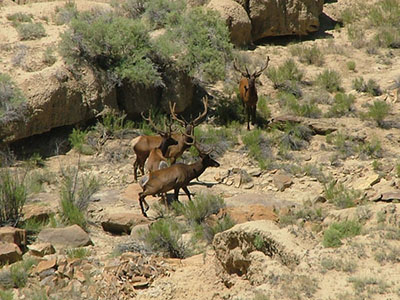
Figure 5. Aerial surveys allow precise evaluation of the age structure of the bull or buck population. Because most wildlife enterprises try to maximize trophy development, knowing the age structure of the population is a key requirement to meeting management goals. (Photo courtesy of E. Watters.)

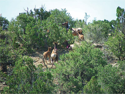
Figure 6. Aerial surveys allow accurate estimation of juvenile:female ratios. Knowing the productivity of a population allows accurate estimates of sustainable yields. (Photo courtesy of E. Watters.)

Sightability models for elk and mule deer have been developed specifically for New Mexico habitats (L. Bender, unpublished data). Detectability of mule deer and elk during helicopter surveys in New Mexico was influenced by a number of factors, including size of groups, amount and type of vegetation cover, and activity. Of these, group size (for both elk and deer) and activity (of deer) had the strongest relationship to detectability. Because detectability was affected by these factors, simple detectability adjustments (e.g., assuming that a constant proportion of the population was consistently seen among surveys) should not be used for management because detectability of elk and mule deer is not constant, but varies based upon animal behavior (grouping patterns and activity). Thus, population estimates and possibly demographic ratios are likely to be inaccurate if not corrected for factors that influence detection of groups.

Sightability models are developed by modeling factors associated with groups seen during surveys versus groups missed. Once developed, sightability models work by predicting the sighting probability (Y) of all mule deer or elk groups encountered, where Y = e^U / 1 + e^U and U = a linear model combining variables influencing group detectability (Hosmer and Lemeshow, 1989). Sightability correction factors (SCF) for each group seen are then developed using SCF = 1 / Y, and the resulting SCF is applied to each group counted during surveys (see discussion in the Estimating Population Size section). The following describes the variables that influenced detection of mule deer and elk groups during surveys in New Mexico and the models that best correct for incomplete detection of individuals. Following this is a walk-through example of how this modeling works for estimating the corrected population size and ratios for mule deer and elk in New Mexico.

Mule deer

The best-supported sightability model for New Mexico corrected for both group size and level of activity:

U = –1.773 + (0.3249 × G) + (0.7689 × A)

where G is the group size and A is a class variable for mule deer activity at the time of observation (when the deer group was first seen from the helicopter) and is coded 1 for moving deer and –1 for standing or bedded deer. Positive coefficients for both group size and increasing activity indicate that detectability of mule deer increases as both group size and degree of movement increase. Sighting probabilities of mule deer groups plateau at >0.99 when group size reaches 22, regardless of group activity. For group sizes of 1 to 22, sighting probabilities vary with both group size and activity, with group size having a proportionately greater effect. During surveys, sighting probabilities for a lone mule deer are approximately 0.10 if bedded/standing and 0.34 if moving. If the group size of mule deer was 10, sighting probabilities increase to approximately 0.67 and 0.90 for bedded/standing and moving deer, respectively. Because mule deer groups are largest in winter, surveys can maximize detectability of mule deer, and thus numbers counted and precision of population estimates, by conducting mule deer surveys in winter when group sizes are largest. This model fit the observed data well and correctly predicted 82% of sighting outcomes during development surveys.

The Mule Deer Sightability Model was developed in varied habitats of north-central (short grassland, piñon-juniper, oakbrush, ponderosa pine, and montane conifer habitats) and east-central (short grassland, piñon-juniper) New Mexico. The model is conservative (i.e., the selected model produces the lowest population estimate among the suite of statistically similar models) in areas with high canopy closure of piñon-juniper or montane conifer forest. For more open habitats, the model is relatively unbiased.

Elk

The best-supported sightability model for elk corrected for group size only:

U = –1.9520 + (0.3546 × G)

where G is the group size. Probability of sighting elk groups increases as group size increases until probability of sighting is >0.99 at a group size of approximately 19. This is true regardless of vegetation type, activity, or other variables that affect sighting of elk during surveys. This model similarly fit the observed data well and correctly predicted 87% of sighting outcomes during development surveys. The Elk Sightability Model was developed in the varied habitats of north-central (sage-steppe, aspen, piñon-juniper, ponderosa pine, montane conifer, montane meadow), northwest (desert scrub, aspen, piñon-juniper, montane conifer), and south-central (desert shrub, oakbrush, piñon-juniper, aspen, ponderosa pine, montane conifer) New Mexico. Like the Mule Deer Sightability Model, the Elk Sightability Model will be conservative in areas with high canopy closure of piñon-juniper or montane conifer forest.

Conducting Surveys

Sightability surveys should ideally be flown using a Bell 206B JetRanger or 206L LongRanger helicopter with a pilot and at least two observers, although similar four-seat helicopters (e.g., Hughes/MD 500, Robinson R44, etc.) likely will not significantly affect model predictions. The lead observer of the survey crew should be located in the front seat beside the pilot, and the secondary observer should be immediately behind the lead observer in the back seat. Surveys can be conducted with or without doors, although without doors greatly enhances comfort during surveys in warmer months.

For total population estimates, survey flights should be flown at 35 to 43 knots and approximately 100 to 150 ft (30–46 m) above ground level. Transect widths should be approximately 0.25 miles (0.40 km). Surveys can be conducted throughout the day, and are generally flown along north–south transects to minimize sun effects on the pilot and lead observer. A GPS track log is extremely helpful to ensure complete coverage of the survey unit.

When located, mule deer and elk groups should be circled and counted, with the following group characteristics recorded for each group.

Mule deer

• Group size.

• Group composition, including numbers of bucks, does, and fawns. Bucks should be further segregated by number of antler points or a subjective yearling, young (raghorn), or mature buck classification. At a minimum, yearlings and older bucks should be distinguished to help differentiate mortality rates and male age structure (Bender, 2006, 2011, 2020b).

• Activity of the first mule deer observed in the group (the one that caught your attention when you first sighted the group), classed as either bedded, standing, or moving.

Elk

• Group size.

• Group composition, including numbers of bulls, cows, and calves. Bulls should be further segregated by number of antler points or a subjective yearling, young (raghorn), or mature bull classification.

If you are only doing herd composition counts (rather than attempting a population estimate), groups of elk or deer counted should still be corrected for sightability if flown outside of the autumn breeding season, which is the only time sexes and age-classes are freely intermixed and thus can yield accurate ratios (Bender, 2006, 2020b). Flights for ratio data only do not have to follow the 0.25-mile transect grids outlined previously.

Estimating Population Size

The following is a simple example of applying the New Mexico Mule Deer Sightability Model to survey data. After completing a survey of the entire ranch, a manager observed 3 groups of mule deer (Table 1) and estimated the population size by using the Mule Deer Sightability Model (available as an Excel spreadsheet at the Corona Range and Livestock Research Center’s website at coronasc.nmsu.edu under the “Mule Deer” link under “For Wildlife Managers”). The following shows how the groups of deer are corrected for groups missed by the sightability model.

The first 3 groups observed in a mule deer survey consisted of 1 running yearling buck (Group 1), 5 standing deer (3 does and 2 fawns; Group 2), and 4 running deer (3 does and 1 mature buck; Group 3).

Applying the sightability model (U = –1.773 + [0.3249 × G] + [0.7689 × A]) results in:

Group 1: U = –1.773 + (0.3249 × 1) + (0.7689 × 1) = –0.6792

Group 2: U = –1.773 + (0.3249 × 5) + (0.7689 × –1) = –0.9174

Group 3: U = –1.773 + (0.3249 × 4) + (0.7689 × 1) = 0.2955

The probability of sighting each group (Y) is then calculated:

Group 1: Y = e^-0.6792 / 1 + e^-0.6792 = 0.336

Group 2: Y = e^-0.9174 / 1 + e^-0.9174 = 0.285

Group 3: Y = e^0.2955 / 1 + e^0.2955 = 0.573

Sighting correction factors (SCF) for each group are then calculated:

Group 1: SCF = 1 / Y = 1 / 0.336 = 2.98

Group 2: SCF = 1 / Y = 1 / 0.285 = 3.51

Group 3: SCF = 1 / Y = 1 / 0.573 = 1.75

The observed deer groups are then corrected for missed groups based on the probabilities of detecting a group with those group size and activity characteristics:

Group 1: 1 × 2.98 = 2.98

Group 2: 5 × 3.51 = 17.51

Group 3: 4 × 1.75 = 7.00

The final population size is estimated by summing all corrected group sizes:

n = Group 1 + Group 2 + Group 3 = 3 + 18 + 7 = 28

In this simple example, the original (uncorrected) survey counted only 10 deer in the 3 groups observed. Because detection of deer during surveys is not 100%, but rather varies with differing group sizes and levels of activity, the corrected total was 28 deer; the survey missed about 18 deer based on the characteristics of groups seen. Thus, if the observed count was used, managers would have greatly underestimated the number of deer on the ranch. Consequently, management decisions based on deer density, such as amount of forage needed or how much to feed if supplementing the deer population, would also have been greatly underestimated. The result could have been much lower animal quality because resources available per individual deer would have been overestimated from the observed count, or a much lower sustainable harvest than was actually available from the population.

Finally, this simple example covered only population size. As shown in Table 1, herd composition ratios would also have been biased using the observed count data. In this example, numbers of bucks would be overestimated (corrected buck:doe ratio = 30:100; uncorrected = 33:100) using the uncorrected observed count data, and the age structure of the bucks would be overestimated (i.e., there were actually proportionally fewer mature bucks than the count data indicated; corrected percent yearling bucks = 63%; uncorrected = 50%). Remember, ratio data, such as male:female, young:female, and age structure data, can provide managers with key information on their populations, including mortality rates and maximum sustainable harvests (Bender, 2006, 2011, 2020b).

As noted previously, to aid in these calculations, a spreadsheet for estimating numbers of mule deer and elk using the New Mexico Mule Deer and Elk Sightability Models is available on New Mexico State University’s Corona Range and Livestock Research Center’s website
(coronasc.nmsu.edu) by clicking the “Mule Deer” link under “For Wildlife Managers.”

Some General Considerations for Surveys

A good survey depends upon good observers, weather (low wind, ideally slightly overcast skies, etc.), and a good pilot. Given these, the following are some further considerations.

• Surveys should cover the entire ranch. Although subdividing the range into survey units (quadrats) and randomly sampling quadrats could reduce flight time and survey expense, the variance associated with sampling error greatly increases the uncertainty in estimates and thus often lowers the precision associated with population estimates below levels needed for accurate management. In other words, the confidence intervals around the mean population estimate will be wider if sampling only a portion of the survey units (quadrats) instead of all.

• Surveys should be conducted when group sizes are largest in order to increase numbers counted and counteract any potential problems associated with small group size correction factors (this is particularly true for bedded mule deer). This generally occurs in the winter, when deer and elk are either concentrated on winter ranges or more closely associated with water in desert habitats. Conducting surveys during this time results in higher sighting probabilities and thus less error associated with model estimates.

Some Comments On Statistical Error In Estimates

Estimates of population sizes and herd composition ratios are just that—estimates. Therefore, they contain error, which is usually fairly minimal if the entire ranch is surveyed, but can be significant if ranches are divided into quadrats and only a sample of the quadrats are flown. Because error in estimates can be difficult to understand, most managers will (and should) treat the mean estimates from the model as a population index and recognize that there is error in the estimates; thus, they are best treated as relative values rather than absolute. In other words, the population estimate of 28 mule deer in the previous example should be viewed as “about 28 or so” or maybe “25 to 30,” and the uncertainty in the value should be considered when making management plans.

The exact error in estimates can be calculated if managers desire (see Cogan and Diefenbach, 1998, and Bender and Spencer, 1999, for the best methods to do this). Three types of error occur in sightability estimates: (1) detectability (visibility) error due to differences in animal detectability (this is what the sightability models try to directly address), (2) model error due to error in regression model (U) estimates, and (3) sampling error due to non-uniform distribution of animals on the landscape. If a population is sampled rather than doing a complete survey, meaning that only a portion of the range/ranch is surveyed and results are extrapolated to the remainder of the area, sampling error contributes the most variance to population estimates (approximately 75–80%), followed by detectability error (15–20%) and model error (<5%; Otten et al., 1993). Alternatively, if the entire area is surveyed, then detectability error contributes the greatest variation to estimates (approximately 90%), followed by model error (approximately 10%; Cogan and Diefenbach, 1998).

Detectability error occurs due to differing visibility among individuals/groups, resulting in some being seen during surveys and others missed (Steinhorst and Samuel, 1989). Because correction factors for missed groups used in sightability models are estimates and not absolute values, this introduces some error into the population estimates. Detectability error can also include counting errors, such as misclassifying animals, undercounting, or overcounting groups (Cogan and Diefenbach, 1998). Most commonly, counting error involves undercounting groups, which introduces a negative bias into sightability models (Cogan and Diefenbach, 1998). As noted previously, detectability error can be minimized by conducting surveys when social group sizes are largest and use of open habitats greatest.

Model error is the variation in the regression predictions of group sizes (Steinhorst and Samuel, 1989). Correction coefficients for variables affecting detectability each have associated error, and thus each detectability-adjusted estimate of group size is precisely that—an estimate, not a point value. The magnitude of model error depends upon the variability in data used to develop the sightability model, sample sizes used to develop the model, and number of variables included in the model. Typically, models with few variables built on larger sample sizes minimize model error (Wong, 1996). Model error is usually negligible compared to detectability and sampling error.

Sampling error is generally the largest error component in sightability models. Sampling error occurs because of a lack of uniformity in the spatial distribution of animals, i.e., the uneven distribution of animals within and among sampling units (quadrats) (Steinhorst and Samuel, 1989). Often, not all sampling units are flown; rather, a subset (often stratified by expected density of elk or deer into strata of high, medium, and low density) is randomly selected and surveyed. The results of these are then extrapolated to all high-, medium-, and low-density strata for a total population estimate. The variation in estimates among surveyed units within a stratum is the sampling error. Because elk and deer are never uniformly distributed across a landscape, differences in numbers among sampling units can contribute significant error to sightability model predictions. Usually, more error is associated with lower-density strata due to patchy, infrequent occurrence of individuals within these strata. Thus, optimal allocation is usually employed for determining numbers of sample units in each stratum needing to be surveyed (Otten et al., 1993). Optimal allocation involves looking at or estimating sampling error within each stratum relative to numbers of animals seen in each stratum, then determining a proportional sampling effort that minimizes total error across strata in the final survey result. An alternative, and perhaps better, solution uses the distribution and numbers of animals counted in each sampled quadrat to incorporate actual distribution of animals into population estimates using a spatial interpolation method known as kriging (Ver Hoef, 2008).

For most wildlife enterprises, the best option to minimize error in population estimates is to eliminate sampling error completely by surveying the entire ranch. This results in only detectability and model error being present in estimates, both of which are usually minor, particularly given that the New Mexico Mule Deer and Elk Sightability Models use few predictor variables and were built from relatively large samples. Therefore, it is highly recommended that managers survey their entire ranch. However, if the ranch is only sampled, then randomization (bootstrap) methods, in preference to normalized variance estimators, should be used to generate comparative confidence intervals for sightability model estimates (Cogan and Diefenbach, 1998; Bender and Spencer, 1999). This will allow better accounting for amount and distribution of error in population estimates (Cogan and Diefenbach, 1998; Bender and Spencer, 1999) from all sources, especially detectability and sampling error.

Acknowledgments

I thank R. Baldwin, J. Boren, A. Darrow, and B. Hoenes for constructive reviews of this circular. Funding was provided by New Mexico State University’s Agricultural Experiment Station, Cooperative Extension Service, and Corona Range and Livestock Research Center; the Santa Fe Trail Mule Deer Adaptive Management Project (STAMP); the New Mexico Department of Game and Fish; the Rocky Mountain Elk Foundation; and multiple private landowners throughout New Mexico.

Literature cited

Anderson, Jr., C.R., D.S. Moody, B.L. Smith, F.G. Lindzey, and R.P. Lanka. 1998. Development and evaluation of detectability models for summer elk surveys. Journal of Wildlife Management, 62, 1,055–1,066.

Bender, L.C. 2006. Uses of herd composition ratios in ungulate management. Wildlife Society Bulletin, 34, 1,225–1,230.

Bender, L.C. 2011. Basics of trophy management [Guide L-111]. Las Cruces: New Mexico State University Cooperative Extension Service.

Bender, L.C. 2020a. Guidelines for monitoring big game populations in New Mexico II: Trend indices [Circular xxx]. Las Cruces: New Mexico State University Cooperative Extension Service.

Bender, L.C. 2020b. Using population ratios for managing big game [Circular 669]. Las Cruces: New Mexico State University Cooperative Extension Service.

Bender, L.C., and R.D. Spencer. 1999. Estimating elk population size by reconstruction from harvest data and herd ratios. Wildlife Society Bulletin, 27, 636–645.

Caughley, G. 1974. Bias in aerial survey. Journal of Wildlife Management, 38, 921–933.

Cogan, R.D., and D.R. Diefenbach. 1998. Effect of undercounting and model selection on a sightability-adjustment estimator for elk. Journal of Wildlife Management, 62, 269–279.

Heffelfinger, J.R., L.H. Carpenter, L.C. Bender, G. Erickson, M.D. Kirchoff, E.R. Loft, and W.M. Glasgow. 2003. Ecoregional differences in population dynamics. In J.C. deVos, Jr., M.R. Conover, and N.E. Headrick (Eds.), Mule deer conservation: Issues and management strategies (pp. 63–90). Logan, UT: Jack H. Berryman Institute.

Hosmer, D.W., and S. Lemeshow. 1989. Applied logistic regression. New York, NY: John Wiley & Sons.

Keegan, T.W., B.B. Ackerman, A.N. Aoude, L.C. Bender, T. Boudreau, L.H. Carpenter, B.B. Compton, M. Elmer, J.R. Heffelfinger, D.W. Lutz, B.D. Trindle, B.F. Wakeling, and B.E. Watkins. 2011. Guidelines for monitoring mule deer populations. Tucson, AZ: Mule Deer Working Group, Western Association of Fish and Wildlife Agencies.

Lancia, R.A., J.D. Nichols, and K.H. Pollock. 1996. Estimating the numbers of animals in wildlife populations. In T.A. Boukhout (Ed.), Research and management techniques for wildlife and habitats (pp. 215–253). Bethesda, MD: The Wildlife Society.

Otten, M.R.O., J.B. Haufler, S.R. Winterstein, and L.C. Bender. 1993. An aerial censusing procedure for elk in Michigan. Wildlife Society Bulletin, 21, 73–80.

Samuel, M.D., E.O. Garton, M.W. Schlegel, and R.G. Carson. 1987. Visibility bias during aerial surveys of elk in northcentral Idaho. Journal of Wildlife Management, 51, 622–630.

Steinhorst, R.K., and M.D. Samuel. 1989. Sightability adjustment methods for aerial surveys of wildlife populations. Biometrics, 45, 415–425.

Unsworth, J.W., F.A. Leban, D.J. Leptich, E.O. Garton, and P. Zager. 1994. Aerial survey: User’s manual. Boise: Idaho Department of Fish and Game.

Ver Hoef, J. 2008. Spatial methods for plot-based sampling of wildlife populations. Environmental and Ecological Statistics, 15, 3–13.

Wong, C. 1996. Population size estimation using the modified Horvitz-Thompson estimator with estimated sighting probability [Thesis]. Ft. Collins: Colorado State University.

For Further Reading

CR-662: Guidelines for Management of Habitat for Mule Deer: Piñon-juniper, Chihuahuan desert, arid grasslands, and associated arid habitat types
pubs.nmsu.edu/_circulars/CR662/

CR-669: Using Population Ratios for Managing Big Game
pubs.nmsu.edu/_circulars/CR669/

CR-688: Understanding Predation
pubs.nmsu.edu_circulars/CR688/

Lou Bender is a Senior Research Scientist (Natural Resources) with the Department of Extension Animal Sciences and Natural Resources at NMSU. He earned his Ph.D. from Michigan State University. His research and management programs emphasize ungulate and carnivore management, integrated wildlife and livestock habitat management, and wildlife enterprises in the Southwest and internationally.

To find more resources for your business, home, or family, visit the College of Agricultural, Consumer and Environmental Sciences on the World Wide Web at pubs.nmsu.edu.

Contents of publications may be freely reproduced, with an appropriate citation, for educational purposes. All other rights reserved. For permission to use publications for other purposes, contact pubs@nmsu.edu or the authors listed on the publication.

New Mexico State University is an equal opportunity/affirmative action employer and educator. NMSU and the U.S. Department of Agriculture cooperating.

Revised September 2020 Las Cruces, NM