TR-45
Brian H. Hurd and Julie Coonrod
College of Agricultural, Consumer and Environmental Sciences, New Mexico State University
Authors: Respectively, Associate Professor (bhurd@nmsu.edu), Department of Agricultural Economics and Agricultural Business, New Mexico State University, Las Cruces, New Mexico 88003, and Associate Professor (jcoonrod@unm.edu), Department of Civil Engineering, MSC01 1070, University of New Mexico, Albuquerque, New Mexico 87131. (Print Friendly PDF)
Table of Contents
Abstract
Introduction
Climate Variability and Change in New Mexico
Constructing Scenarios for Socio-Economic Trends and Baseline Changes
Estimating the Hydrologic and Streamflow Changes under Climate Change
A Hydro-Economic Model of the Rio Grande
Assessment Results and Findings
Findings and Conclusions
Acknowledgements
References
Abstract
Social, economic, and environmental systems in water-scarce New Mexico and throughout the arid southwest are vulnerable to disruptions in water supplies that are likely to accompany future climate changes. With a particular focus on potential economic consequences for New Mexico, this study uses a hydro-economic model of the Rio Grande watershed to integrate plausible changes in climate with hydrologic responses and water demands, within a framework that optimizes water-use allocations for the greatest economic benefit. The study uses three climate change scenarios across two future time periods selected to represent the range of effects indicted by the outputs across 18 GCMs using the SRES A1B emissions scenario. These six climate change scenarios were then used to model runoff changes using the WATBAL hydrologic model (Yates, 1996), which integrates climate and hydrologic variables, and to change water demand parameters in the hydro-economic model. Primary findings confirm that ecosystems are at greatest risk in New Mexico, followed by agricultural water users, as water is increasingly transferred to maintain urban and industrial users, whose economic productivity is greater. While total annual economic losses are estimated in the vicinity of $300 million, under severe climate changes where runoff is reduced by nearly 30%, both economic and non-economic losses are likely to be significantly higher. This is due primarily to the effects of some strongly optimistic model assumptions, e.g., assuming no conflicts over water rights or water transfers, and to several significant and valuable omissions in the analysis, e.g., the environmental and social services that agriculture and the environment provide.
Introduction
New Mexico has a unique blend of cultures and landscapes, of agrarian values and high-tech economies, of rare ecosystems, fertile valleys, and expansive desert rangelands. It is a place where people have long settled and where growing numbers still long to settle, as migration trends illustrate. New Mexico’s growing communities are praised for their quality of life, climate, and retirement opportunities. The Rio Grande Valley, which bisects New Mexico, has industry, tourism, residents old and new, and agriculture, all of which stake claims to water resources. These water resources must also serve the traditions and economic needs of twenty-three Native American tribes and pueblos, and flow through traditional acequias—canals—felt by many to be the lifeblood of four-hundred-year-old Hispanic communities. The Rio Grande is also home to endangered silvery minnows in the last remnant of their historical habitat and to flocks of migrating cranes and geese who gather in vast numbers to rest and refuge in riparian bosques (woodlands).
The Rio Grande—and the subterranean aquifers that it feeds in some regions—is the principal, often only, water source for cities and farms from Southern Colorado through New Mexico and into far West Texas, as shown in Figure 1. The vulnerability that these water users face together—especially in light of potential climatic and hydrologic changes—is indicated not only by their dependence on a sole source of supply but by the oversubscribed claims to and exhaustive use of this source (Hurd et al., 1999; Hurd et al., 2006). The level of use is so exhaustive of surface supplies that after the thirst is satisfied it is normal for the Rio Grande to merely trickle with salt-laden return flows and summer storm runoff for 180 miles until its confluence with Mexico’s Rio Conchos, just above Big Bend National Park near Presidio, Texas. There, newly reconstituted, it continues a remaining 1,100 miles to the Gulf of Mexico.
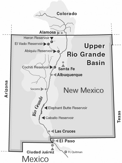
Figure 1. The Upper Rio Grande watershed and study area.
The future health of New Mexico’s economy, cultural traditions, and riparian ecosystems is so tightly hinged, in the long run, to the flows of the Rio Grande that the aim of this study—to monetize the economic consequences resulting from climatic and hydrologic changes—may miss highlighting significant changes in other non-economic but highly valued characteristics. As highlighted by this paper, there are many limitations to our capacity to measure and express even the economic consequences from changes that affect the regional character and economy in such profound ways.
The paper begins with a discussion of New Mexico’s climate and the approaches used to model and identify appropriate scenarios of climate change. Next, the state’s hydrologic situation is described—through review of key studies that have tried to understand climate influences on the state’s rivers, and discussion of the hydrologic modeling used to examine climate change scenarios and estimate streamflow changes. This is followed by a description of the economic approach used to estimate impacts. A hydro-economic model of the Rio Grande watershed is used that optimizes the allocation of available water and, as necessary, readjusts water-use patterns such that economic losses are minimized during, for example, a long-run downturn in streamflow. The final sections of the paper present and discuss key findings and conclusions.
Climate Variability and Change in New Mexico
Tree-ring analysis indicates that New Mexico has a long and highly variable history of precipitation and streamflow, punctuated by periods of high runoff and drought. Nearly five hundred years of Rio Grande streamflow has been reconstructed and is shown in Figure 2. This reconstruction is long enough to illustrate that the period of recorded streamflow, roughly 100 years, does not fully account for the range of natural extremes. For example, neither the recent drought from 2001–2005 nor the 1950s drought—the most severe in recent memory—match the severity of eight or nine previous drought episodes within this reconstructed record. Some anthropologists speculate that droughts in periods even earlier than shown in Figure 2 were severe enough to cause the collapse of early pre-Columbian civilizations in the region (Plog, 1997)1. Such observations indicate that significant climate anomalies are not unprecedented in this region—and plausibly suggest that with continued radiative forcing of the atmosphere caused by greenhouse gases, and rising effects on the earth’s energy balance, there is reasonable expectation of exceeding these natural extremes in the future (IPCC, 2007).
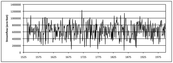
Figure 2. Long-run tree-ring reconstructed streamflow of the Rio Grande near Del Norte. Source: Woodhouse, C.A., et al. 2004. TreeFlow Colorado Streamflow Reconstructions. IGBP PAGES/World Data Center for Paleoclimatology Data Contribution Series # 2004-029. NOAA/NGDC Paleoclimatology Program, Boulder CO, USA.
In assessing climate change impacts, scenarios selected should be based on climate models that reflect the range of plausible regional outcomes. By choosing across the available range, uncertainty about the regional climate change is conveyed more accurately than it would be if selections were narrowly targeted. For example, use of outcomes only from models estimating precipitation increases would be misleading if other models project a decrease. Differences across climate models tend to indicate the minimum uncertainty concerning possible regional climate change. Therefore, to capture the plausible range of climate outcomes associated with continued atmospheric forcing, Smith and Wagoner (2006)—with guidance and technical assistance from scientists at the National Center for Atmospheric Research (NCAR)—selected three climate models from the 18 used in the IPCC’s Fourth Assessment report (IPCC, 2007), choosing those that were most representative of the range of precipitation response from relatively wet to relatively dry, with one approximating the median. In this comparison each climate model used the same underlying greenhouse gas emissions scenario, the Intergovernmental Panel on Climate Change (IPCC) emission scenario referred to as A1B.2 This emissions scenario is generally regarded as “neither too optimistic nor pessimistic,” and is commonly associated with “business as usual” economic activity levels. Furthermore, the spatial resolution of climate model output is coarse relative to the regional scales most of interest, with grid cell sizes covering approximately 5.6° in latitude and longitude, i.e., very large areas of approximately 300 miles across, as shown in Figure 3 for New Mexico. This limitation means that local differences in climate change, for example, by altitude or on the leeward and windward side of mountain ranges is not well represented and contributes uncertainty to the model results.
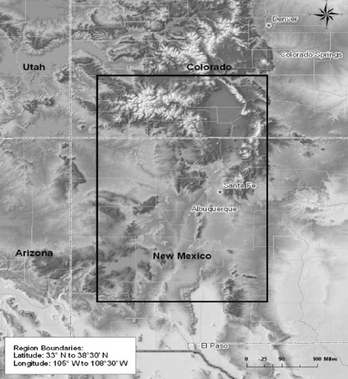
Figure 3. Approximate location of the GCM Grid Cell used to estimate temperature and precipitation changes for the New Mexico climate change scenarios.
Based on this process, the following three climate models were selected to represent the range of outcomes projected for New Mexico:
- Wet: hadcm3 (Hadley Centre for Climate Prediction and Research Met Office)
- Middle: CSIRO (Commonwealth Scientific and Industrial Research Organisation—Atmospheric Research Australia)
- Dry: NOAA (National Oceanic and Atmospheric Administration— U.S. Department of Commerce) GFDL0 (Geophysical Fluid Dynamics Laboratory)
Using the temperature and precipitation outcomes estimated by each of these three models, Smith and Wagner (2006) develop six climate-change scenarios, a Wet, Middle, and Dry scenario for each of two future time periods, a closer time frame, simulating years 2020–2039, and one further, simulating years 2070–2089, referred to in the analysis as 2030 and 2080 scenarios. Figure 4 (panels A through D) illustrates the estimated temperature and precipitation changes for New Mexico under each of the six scenarios.
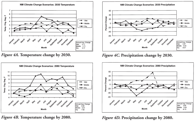
Figures 4A-D. Temperature and precipitation change scenarios for New Mexico. Source: Smith, J.B. and C. Wagner. 2006. Scenarios for the National Commission on Energy Policy. Memorandum to Brian Hurd from Stratus Consulting Inc., Boulder, CO. August 1, 2006.
Constructing Scenarios for Socio-Economic Trends and Baseline Changes
Economies develop, technologies advance, and populations grow and change; together these factors alter the socio-economic setting in which the future climate is realized. In the future, will New Mexico residents, industries, and cultural traditions be more or less vulnerable to a changing climate? Population growth in New Mexico cities—and in cities throughout the southwestern U.S.—has been significant and appears not to be slowing. Studies suggest that this growth amplifies exposure and the vulnerability of these communities to risks from severe droughts and flash floods (Hurd et al., 2006, 1999). As Frank Pinto, the Executive Director for the UNDP’s Global Environment Facility, writes in his forward to a UNDP handbook on developing socio-economic scenarios:
Developing socioeconomic scenarios of the future is important because socioeconomic changes may substantially increase or decrease vulnerability to climate change. For example, as populations grow, human activities that pollute may increase and habitats may be fragmented. Together, these changes may increase the vulnerability of some aspects of human welfare. If the economy grows and technologies can be developed, vulnerability may be reduced in some sectors but possibly increased in others. These interactive changes can be explored (although not predicted) through the development of alternative socioeconomic scenarios of the future (Malone et al., 2004, p. 5).
For accuracy and consistency, estimates of climate change impacts expected sometime in the future should therefore account for and reflect expected changes in baseline population and socio-economic conditions. To construct socio-economic baseline scenarios, Smith and Wagner (2006) collected demographic trend data on population and income growth for New Mexico from the U.S. Census, to which were added additional data from the New Mexico Bureau of Business and Economic Research (NM BBER, 2004) on population growth trends within the counties of the Rio Grande watershed.
Using county-level population growth rate projections developed by NM BBER (2004) for five-year incremental periods out to 2030, annual population growth rates for the counties in the Rio Grande watershed were estimated. The population growth trend was further extrapolated to 2080 by fitting a quadratic trend to the data. The results show that population growth in the Rio Grande corridor is projected to decline fairly steadily over the study period, falling from current annual rates just under 2% to approximately 1% in 2030 and 0.5% by 2080, as shown in Figure 5. To ensure consistency of the population estimates with the SRES A1B scenario used in developing the climate change scenarios, the estimates were compared to those developed by Smith and Wagoner (2006)—which were SRES A1B rescaled U.S. Census estimates—and were found nearly identical at the state level. Figure 6 shows the estimated population in these counties for the years 2000, 2030 and 2080 using the extrapolated growth rates.
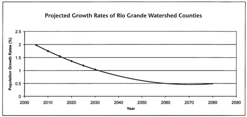
Figure 5. Projected annual growth rates of Rio Grande watershed counties in New Mexico. Source: N.M. Bureau of Business and Economic Research, rev. 2004. Counties include: Bernalillo, Doña Ana, Los Alamos, Rio Arriba, Sandoval, Santa Fe, Sierra, Socorro, Taos, Torrance, Valencia.
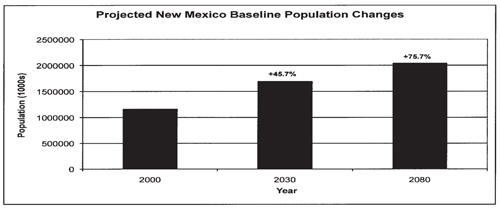
Figure 6. Projected populations of Rio Grande watershed counties in New Mexico. Source: N.M. Bureau of Business and Economic Research, rev. 2004. Counties include: Bernalillo, Doña Ana, Los Alamos, Rio Arriba, Sandoval, Santa Fe, Sierra, Socorro, Taos, Torrance, Valencia.
Estimated population change is the primary driver used to shift aggregate urban water demand in the analysis and to provide an appropriate baseline against which future climate change impacts can be compared. Although per capita income and regional economic development are also expected to increase and contribute to wealth formation over the relevant timeframe, their effect on aggregate municipal and industrial water demand is much less clear than that from population changes. Household water demands can rise with income, reflecting, for example, an increase in the size of homes. However, estimated income elasticities are generally quite low and to a significant degree are expected to be offset by improvements in household water-use efficiency.
Estimating the Hydrologic and Streamflow Changes under Climate Change
Estimating changes in streamflow and water availability is the result of hydrologic simulation of the climate change scenarios. These simulations are run using the conceptual rainfall–runoff model called WATBAL, which simulates changes in soil moisture and runoff as a result of changes in temperature and precipitation (Yates, 1996, 1997). WATBAL is conceptualized as a one-dimensional water balance model composed of two elements. First is a water balance component that describes water movement into and out of a basin consisting of three sub-processes describing i) surface runoff, ii) sub-surface flow and iii) maximum catchment water-holding capacity. The second models the system energy balance and uses the Blaney–Criddle relationship to simulate evapotranspiration (FAO, 1992) and to model the snow storage and runoff. Parameters in WATBAL include the size of catchment areas and the rate of water additions and removals, which are based on historical runoff relationships, calibrated changes, physical characteristics, and input data such as monthly rainfall and temperature. Water is added by precipitation, can be accumulated to some extent, and is removed by evapotranspiration, surface runoff or sub-surface runoff.
The simplified representation of soil moisture dynamics has been shown to adequately represent runoff changes due to climate fluctuations (Yates and Strzepek, 1994; Yates, 1996, 1997). WATBAL was applied to each catchment area in the Rio Grande watershed to simulate runoff and streamflow such that it is spatially and temporally consistent with the hydro-economic model described in the next section.
For each watershed corresponding to the hydro-economic model (see Figure 7), historical monthly values for streamflow, precipitation, and temperature were required. Monthly streamflow values are available from the USGS (waterdata.usgs.gov). Historical precipitation and temperature grids (4 km grid cells) are available for the contiguous United States from the PRISM group (www.ocs.orst.edu/prism). The historical 30-year climatic period of 1971 to 2000 was chosen. This period of time contains some of the wettest years on record. However, this period of time also has the most complete record. Any 30-year climate period will contain sufficient variability to calibrate WATBAL, but the calibrated models for the same basin will differ based on the climate period selected.
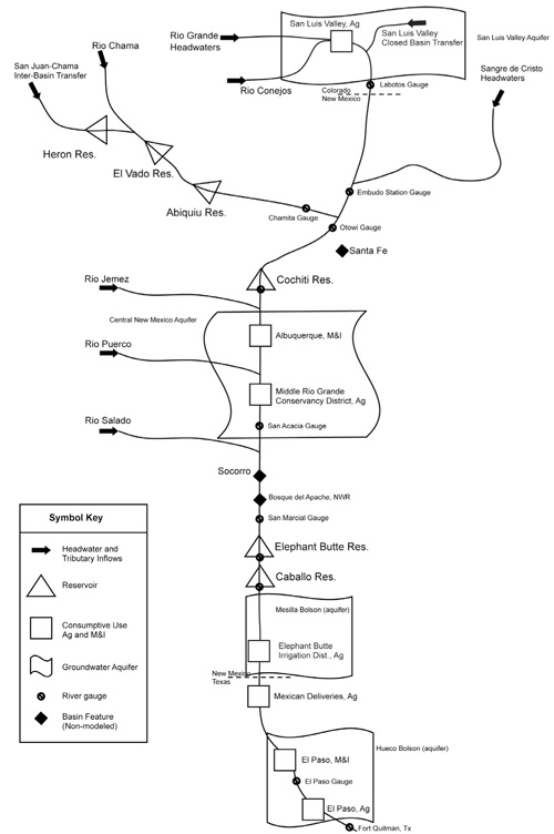
Figure 7. Schematic diagram of the Rio Grande hydro-economic model.
Downloading streamflow data is straightforward, as the data correspond to a single point. Conversely, precipitation and temperature are spatially distributed across the watersheds that drain to the gauge locations. From the PRISM website, 1,080 monthly data files were extracted: 360 precipitation, 360 maximum temperature, and 360 minimum temperature files for 1971–2000. Each file contained data for the entire contiguous United States (Doggett et al., 2004). ArcGIS was used to create watershed zones based on the contributing areas of the gages selected to be modeled. These zones were then used with ArcGIS to spatially average the precipitation and temperature over the watershed for each gage. As this procedure was required for each of the 1080 files, the process was automated by writing a Python script that could be used in ArcGIS to convert the PRISM file grids to rasters, clip the rasters to the watershed zones, and calculate average values across the watersheds. The ArcToolbox>Spatial Analyst Tools>Extraction>Sample tool was then used to extract a DBF table of the attributes for each of the spatially averaged grids. Using Excel, the ArcGIS output files were arranged and consolidated by watershed. The average monthly temperature was calculated by averaging the maximum temperature and minimum temperature for every month. This method was validated by researchers at the University of Dayton, who studied 53,004 daily temperature records (http://academic.udayton.edu/kissock/http/Weather/default.htm).
WATBAL was calibrated for each individual watershed using the historical data (monthly values for streamflow, spatially averaged precipitation, and spatially averaged temperature.) The future climate change scenarios were applied to each watershed to obtain possible 30-year scenarios of monthly values for precipitation and temperature for each watershed. WATBAL was then used to estimate the corresponding monthly values of streamflow associated with each climate scenario for each watershed.
A Hydro-Economic Model of the Rio Grande
Modeled runoff and streamflow, the principal outputs from the hydrologic model, are key drivers in estimating changes in water use and allocation, aquifer and reservoir storage, and changes in economic welfare. These changes were estimated using a river-basin scale hydro-economic model (RBHE) of the Rio Grande watershed which simulates the management of water systems from a watershed-wide perspective. The model optimizes the allocation, use, storage, and management of available water such that the greatest long-run economic benefits are achieved within the legal boundaries of river compacts and treaties and with available resources, technologies, and infrastructure.
One of the key aspects of the RBHE model is the explicit treatment of the underlying value of water, often represented as mathematical functions that relate the marginal economic value of water to the quantity of water use, i.e., “water demand functions.” By specifying this relationship, the modeler is implicitly specifying the flexibility of the particular water user to changes in water prices. Economists often refer to this as the “price elasticity of demand”—in other words, how the quantity of water use changes in percentage terms to a percentage change in price. As climate change interacts with economic markets by affecting resource supplies and demands, ultimately resource prices are altered and signal to water users that a change in water use is indicated—providing that institutions and policies permit the direct and transparent relay of these implicit prices to water users. Adaptation to a water shortage, for example, occurs as some water users less tolerant of price increases begin to curtail their use.
Hydro-economic models have several advantages for long-term planning and assessment over alternative models of the water-budget and system-simulation type. First, by using an optimization framework RBHE models replicate an active decision environment that explicitly recognizes the opportunity costs and economic tradeoffs inherent in any given water allocation and storage decision. Second, simulation and water budget models use a “what if” perspective to assess the consequences that would follow from a given allocation decision; however, only an optimization framework can systematically sift through all the permutations of possible allocation decisions and identify those that are potentially “best” and worthy of closer scrutiny. This is a distinct advantage when examining and comparing the effects of large-scale, system-wide changes, especially if behavior within the system is dynamic and roughly follows the optimization objectives. Third, RBHE models provide explicit information regarding the value of water, how it is affected by water supply changes, how it varies both temporally and spatially, and how it is altered by physical limitations and institutional constraints. As a result, RBHE models excel in their capacity to identify strategies that can improve water-use efficiency, infrastructure designs, investment decisions, and institutional arrangements.
Vaux and Howitt (1984) pioneered the development and use of RBHE models for regional water assessment in examining water transfer issues in California. Booker and Young (1991, 1994) extended the approach by more realistically capturing the extensive network characteristics of a watershed in their study of the Colorado River basin. More recently, climate change impacts have been assessed by Hurd et al. (1999, 2001, 2004), and in California by Tanaka et al. (2006) using the RBHE model approach. In the upper Rio Grande basin, Ward et al. (2001) developed an RBHE model and used it to examine the consequences of sustained drought; this was further extended by Ward et al. (2006) to assess the combined effects of drought and endangered species protection on the water economy of the Rio Grande. Descriptions of the conceptual foundations and use of RBHE can be found in Hurd (1999, 2004), Null and Lund (2006), JWRPM (2006), Draper et al. (2003), Jenkins et al., (2004), and in Cai et al. (2003).
This study builds on the Rio Grande hydro-economic (RGHE) model of Ward et al. (2001) by making several important modifications, the most important of which is the reduction in time-step from annual to monthly. By increasing the temporal resolution to monthly, the RGHE is better able to capture the effects of an expected shift in the streamflow hydrograph toward an earlier snowmelt and peak runoff as a result of climate change. This extension also improves the model’s capability to simulate changes in seasonal water use patterns, instream flow requirements for endangered species, and recreational use patterns at reservoirs.
As with all hydro-economic models, the RGHE model is oriented towards economizing available water resources by identifying the most valued use and storage, conveyance, and water quality decisions possible within the existing physical, institutional and infrastructural limitations. In addition, two important behavioral assumptions implicit in the modeling framework can significantly affect the nature and interpretation of the results. First, competition between water users is assumed, and furthermore, these water users aim to maximize their expected net economic returns. This implies that water is freely transferable across uses with no restrictions or transaction costs, and is subject only to the physical and institutional restraints of the system (i.e., logical mass–balance relationships must be satisfied between the flows of water from upstream to downstream locations and between adjacent time-periods in storage conditions). By ignoring the significant transactions costs of water transfers and, indeed, some of the underpinnings of the institution of prior appropriation in defining water rights, the model understates the economic costs of adjustment and adaptation to changing water supplies. Another artifact of this assumption is that the optimization framework is not necessarily a “good” predictor of current and actual patterns of water use. This limitation, however, does not detract from the insightful and useful results, which focus less on the absolute level of economic output and instead focus on the magnitude of change—a measure that is likely to be more robust (Draper et al., 2003; Tanaka et al., 2006).
Second, the model design allows for “perfect foresight” across the 30-year sequence of runoff and streamflow conditions. By assuming away future uncertainty in runoff and streamflow, adjustments and adaptations—in the form of storage and use decisions—are optimally executed without errors in the amount or timing of adjustment. As a result, this assumption contributes further to the model tendency to understate economic adjustment costs and hence the economic impacts of water supply changes under climate change.
A conceptual diagram of the model is given in Figure 7, which depicts key physical characteristics of the watershed, including tributaries, inflows from the hydrologic model outputs, return flows from users, diversion points, and reservoirs. The model is developed and executed using the General Algebraic Modeling System (GAMS, Brooke et al. 1988). In summary, the model consists of:
- A nonlinear objective function that aggregates all the sources of economic value and cost in the watershed as a function of water use and reservoir storage, including the cost of pumped groundwater, the benefits associated with reservoir recreation, and the shifting water demands due to population and climate changes. Figures 8a and 8b illustrate the urban sector aggregate and household benefit functions, respectively. Figures 8c and 8d show examples of the aggregate and per acre functions for the agricultural sector. Figure 8e shows net economic benefits for flatwater recreation on reservoirs as a function of storage level.
- A system of linear constraints that characterize:
- Spatial network and streamflow continuity of monthly runoff into the basin, main stem and tributary streamflow, surface water diversions, and sub-basin water transfers, i.e., where water enters the system, how it travels and is distributed, where it is used, and how it leaves the system.
- Inter-temporal balances in reservoirs and aquifers between adjacent time periods (i.e., months), and mass-balances within each time period that balance additions and extractions, including storage releases and evaporation losses.3
- Institutional limitations of compacts, treaties and intergovernmental agreements, for example, the Rio Grande Compact between Colorado, New Mexico and Texas; the 1906 Treaty with the Republic of Mexico requiring the annual delivery of 60 kaf/yr; and operational rules between the Elephant Butte Irrigation District (EBID) and the El Paso Water Conservancy District #1 (EPWCD# 1). See Ward et al. (2001) for details.
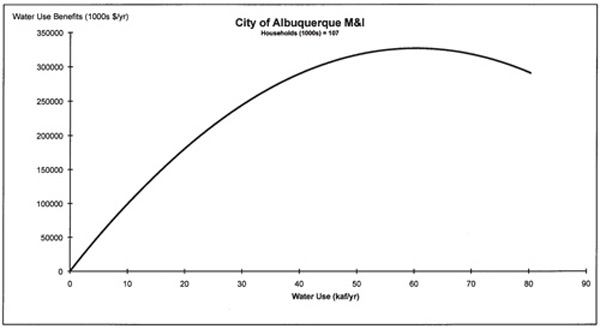
Figure 8A. Example of a municipal and industrial (M&I) aggregate benefit function.
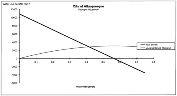
Figure 8B. Example of annual household water demand and total net benefits.
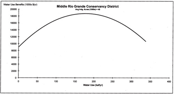
Figure 8C. Example of an agricultural aggregate benefit function.
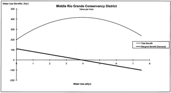
Figure 8D. Example of annual agricultural water demand and total net benefits per acre.
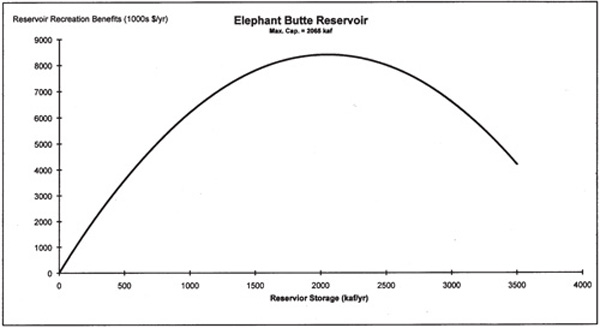
Figure 8E. Example of total benefits from reservoir flat-water recreation.
Figures 8A-8E. Examples of economic benefit functions in the RGHE model.
Incorporating the Climate Change and Socio-Economic Baseline Scenarios into the Rio Grande Hydro-Economic Model (RGHE)
In modeling the climate change and socio-economic baseline scenarios previously described, several key changes in the model inputs and parameters are highlighted that coincide with changes in scenarios and, in the process, introduce the scenario terminology that is used subsequently to report the key results and findings.
A total of nine scenarios were run using the RGHE model. Three baseline scenarios were modeled without the effects of climate change but with the projected changes in population and its attendant shift in urban water demand, referred to as: 2000 Baseline, 2030 Baseline, and 2080 Baseline. In addition, six climate change scenarios were run, one for each of the combinations of the three representative climate change patterns and the two time periods, referred to as: 2030 Dry, 2030 Middle, 2030 Wet, 2080 Dry, 2080 Middle, and 2080 Wet. In presenting the results, the relative effect of each climate change scenario is compared against the appropriate baseline time period, for example, all 2030 climate scenarios are compared against the 2030 baseline using the same population change assumptions.
Key changes in model inputs and parameters across the climate change and socio-economic baseline scenarios are summarized below:
- Streamflow and runoff input is altered. Using the output from the hydrologic simulations, the 30-year sequence of monthly runoff for each inflow point is modified according to the selected climate change scenario.4
- Reservoir evaporation rates are changed. Using estimated changes in potential evapotranspiration rates from simulating the energy-balance changes in the WATBAL hydrologic model, adjustments are made to the monthly water losses for each reservoir in the upper, middle, and lower watersheds under each climate change scenario, as shown in Figures 9a through 9f.
- Agricultural consumptive water use is shifted. Reflecting the increased irrigation requirements associated with higher temperatures, consumptive agricultural water demands are raised consistent with agronomic needs but without implying an increase in net economic benefits.5 The assessment implicitly assumes changes in the mix of crops grown—consistent with current crop technologies. There are many changes in New Mexico agriculture that are plausible over the next 50 years, including changes in genetic technologies and crop yields, incidence of pests and diseases, and loss of arable land due to urban development. Each of these changes could alter the agricultural demand and value of water; however, owing to the speculative nature of these changes they are not included in the present analysis.
- Urban water demands shift in response to population changes. Population change is accounted for in each scenario that is run in a future time period, either for the 2030s or 2080s. These changes result in an increase in aggregate household water demand and, hence, in the estimated value of economic services generated. Although landscape irrigation requirements for non-native grasses would be expected to rise in parallel with agricultural demands, these increases would be expected to be offset by improvements in household water-use efficiency and in continued trends of reduced turf landscapes.6 Therefore, in the present analysis, household water demand is assumed to be invariant to climate changes. It should be noted that there are many issues related to urban water use that can be expected to affect urban water demands and values over the coming 50 years, such as water re-use and recycling and availability of alternative water supplies from, for example, desalination of extensive brackish aquifer resources. These new strategies, which would increasingly be turned to as water prices rise, are not included in the present assessment; they would, if implemented, most likely reduce some of the net economic impacts estimated in this study.
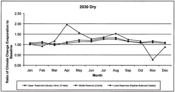
Figure 9A. 2030 Dry evaporation rates.
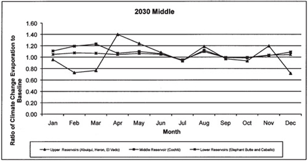
Figure 9B. 2030 Middle evaporation rates.
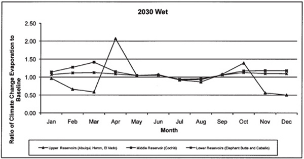
Figure 9C. 2030 Wet evaporation rates.
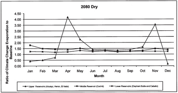
Figure 9D. 2080 Dry evaporation rates.
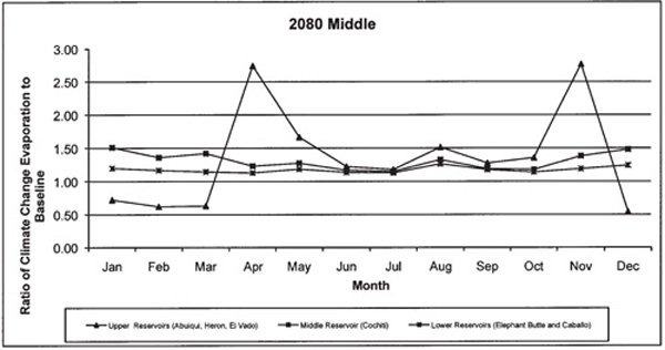
Figure 9E. 2080 Middle evaporation rates.
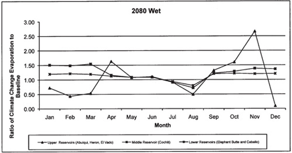
Figure 9F. 2080 Wet evaporation rates.
Figures 9A-9F. Relative change in regional monthly reservoir evaporation across the six climate change scenarios.
Endangered Species Concerns
The Rio Grande, especially the Middle region between Cochiti and Elephant Butte Reservoirs, is the last remaining habitat for the endangered Silvery Minnow. As a result, the U.S. Fish and Wildlife Service (USFWS) has determined that a minimum instream flow of 50 cfs is necessary at the San Acacia gauge for species protection. Aggregating this flow level into a monthly estimate and using a 100% safety factor to account for daily variability results in a streamflow minimum of 6 kaf/month. This constraint is maintained in the analysis all model runs.
Assessment Results and Findings
WATBAL and the RGHE model were run to simulate and optimize the management of a 30-year sequence of monthly streamflows for each of three baseline scenarios (2000 Baseline, 2030 Baseline, and 2080 Baseline) and for each of the six climate change scenarios (2030 Dry, 2030 Mid, 2030 Wet, 2080 Dry, 2080 Mid, and 2080 Wet). Model results are presented and described in the first two sections below. This is followed by a section summarizing the possible effects of model assumptions, uncertainties, and notable omissions, cautioning against the unqualified use of the estimated impacts from the models alone.
Streamflow and Hydrologic Assessment
Consistent with the RGHE model schematic shown in Figure 7, WATBAL modeled streamflows for each of seven tributary inflows within the Rio Grande watershed (in addition, two inter-basin transfer inflows are also included but are not assumed to vary, as described in footnote 6). The most important tributary inflow to the Rio Grande is the mainstem headwaters coming from the San Juan Mountains of southern Colorado and passing the river gage at Del Norte, accounting for more than 35% of annual streamflow. The relative contribution of each of the seven modeled tributaries is shown in Figure 10, which also highlights the peak streamflow months of May and June under current climate. Most of the flow in the Rio Grande is the result of snowmelt in the higher elevations during late spring. Flow from the Rio Puerco and Rio Salado is mostly driven by July and August monsoons. These rivers are perennial and quite erratic in nature. A monthly time step cannot adequately represent perennial streams, as flow is event-driven, yet monthly time does account for the time periods when the Puerco and Salado have been responsible for consistent increased Rio Grande flows.
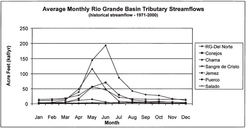
Figure 10. Average monthly streamflow for the Upper Rio Grande Basin tributaries under Baseline conditions (Historical period: 1971–2000).
To see how climate change might affect the streamflow hydrograph, average monthly streamflows for each tributary were aggregated and plotted for each scenario as shown in Figure 11. Two results show clearly in this figure. First, peak flow and total streamflow decline for all of the climate change scenarios, whether or not they are relatively “wet.” The apparent robustness of this result could have important implications for the management of water resources in the region. Although there is a potential for summer monsoonal activity to increase, as suggested by the 2080 Wet scenario, this is not likely, according to the model results, to offset the losses from diminished snowpack in the headwater regions. Second, there is a pronounced shift in later periods (i.e., 2080s time frame) in the peak runoff month—it shifts by about 30 days. In all of the 2080-period runs, the peak occurs in April and, perhaps equally as important, there is a significant increase in late winter runoff compared to under current conditions.
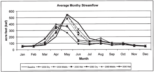
Figure 11. Average aggregate streamflow by month for each climate change scenario.
To further illustrate potential changes in the relative likelihood of basin streamflow, Figure 12 presents the total runoff data for each scenario in the form of a cumulative probability function. This figure shows, for example, the substantial change in the distribution of runoff between present and changed climates. The severe dryness of the 2080 Dry scenario is apparent in the figure where median runoff drops by nearly 1/3, from approximately 1.6 maf/yr to less than 1.1 maf/yr.7
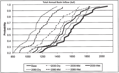
Figure 12. Cumulative distributions of total basin streamflow across the climate change scenarios.
With the hydrograph shift indicating lower runoff totals and a shift toward a greater share of runoff occurring earlier, i.e., reflecting both an earlier snowmelt and lower snowfall totals, water availability during peak use periods is likely to be significantly more dependent on stored water management in reservoirs and aquifers than at present. The results of the RGHE model below show further implications of these possible changes in water availability.
Assessment of Water Use and Economic Impacts
As illustrated by the changes in both amount and timing of annual snowmelt and runoff, there is a significant potential for climate change to disrupt the current allocation and management of New Mexico’s water resources. How these changes might affect current and future water users is the primary focus of the hydro-economic model—the model highlights adaptive changes in allocation and storage, within the existing infrastructure and technology, to minimize disruption and economic losses to the region as a whole. The assessment results are presented in two sections. First modeled changes in consumptive use are described, highlighting shifts in allocation between agriculture and urban use by scenario. The second section presents the estimated economic effects of these changes in allocations and patterns of use by scenario.
Changes in Water Use and Allocation. As might be expected for water use in a basin that exhausts even the present water supply in normal years, any reduction in long-run, average supply necessarily leads to a reduction in long-run average use. Figure 13 shows the modeled changes in aggregate water use across the scenarios. Heavily influenced by the pattern of agricultural irrigation that peaks in June, the figure shows how total water use is curtailed as total supplies diminish with the severity of climate change. The dry scenarios lead to declines in total water use of nearly 10% and over 25% for the respective periods of 2030 and 2080. Declines of 2% and 18%, respectively, for 2030 and 2080, accompany the middle scenarios and declines of nearly 4% and 6.3% the wet scenarios. Note that the “middle” scenario is wetter than the “wet” scenario in the earlier (2030) time period, thus explaining the estimated higher loss of 4% for the wet scenario compared with 2% for the middle scenario.
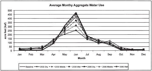
Figure 13. Average monthly aggregate water use for each climate change scenario.
As stated earlier, hydro-economic models are very adaptively efficient—they anticipate water supply changes perfectly and execute allocative changes with perfect timing and efficiency. As a result, the modeled changes in water use by sector will strongly reflect differences in the relative economic value of water in each sector. These differences are most strongly evidenced in Figure 14, which shows the modeled changes in streamflow, agricultural sector, and urban sector allocated use, by climate change scenario. For all but the two most severe scenarios, reductions in modeled water allocation and use are less than reductions in streamflow. For example, in the 2030 dry scenario, streamflow falls by nearly 14%, which leads to a drop in agricultural use of 12% and in urban water use of 0.3%. Each of the wetter scenarios—2030 middle, 2030 wet, and 2080 wet—results in virtually no allocated reductions to the urban sectors, with agriculture absorbing the reduction in runoff nearly entirely. Each of the two drier scenarios—2080 middle and 2080 dry—shows quite significant reductions in agriculture and to some degree in urban water use.
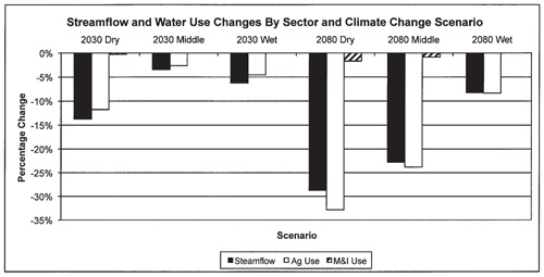
Figure 14. Streamflow and water use changes by sector and climate change scenario.
As expected, these results illustrate the relatively high modeled demand for urban water as compared to agricultural water, as evidenced by the example demand curves shown by Figures 8b and 8d, respectively, and the high share of agricultural water use in the Rio Grande basin, approximately 87.5% in the modeled baseline year of 2000.
Reductions in modeled runoff and water supply are not equally shared across water users. Rather, by considering the relative economic contribution of water users, reductions are allocated to minimize long-run expected losses to total regional economic production. In other words, the optimization framework used here enables the system, by assigning reductions to certain sectors, to avert potentially much greater economic losses that would follow if water use reductions were necessary in other, non-agricultural economic sectors.
Estimated Changes in the Marginal Value of Water. From an economic perspective, a rising price is the clearest signal of increasing relative scarcity. Water resources in New Mexico are increasingly scarce as a result of two processes—increasing demands from growing populations and, potentially, falling water supplies given the estimated effects of climate change. Both effects are evidenced in Table 1, which shows the change in the marginal value (i.e., modeled price) of water at two points in the watershed, the Rio Grande headwaters in Del Norte, Colorado and the Sangre de Cristo headwaters in Northern New Mexico. The estimated values for Colorado are much higher than for New Mexico as a result of the Rio Grande Compact and the relatively high value of agricultural production in the San Luis Valley. For New Mexico, the Sangre de Cristo values are much more representative of the marginal value of water, which is primarily measured by its marginal value for agricultural uses.
Table 1. Estimated Value of Rio Grande Water by Climate Change Scenario
| Climate Change Scenario |
% Change Average Annual Runoff |
Marginal Value of Water in Rio Grande Headwaters* $ per acre foot (% difference from baseline) |
|
| Rio Grande Del Norte (Colorado) |
Sangre de Cristo (New Mexico) |
||
| 2000 Baseline | $66.82 (0%) |
$17.23 (0%) |
|
| 2030 Baseline | (0%) | $67.40 (0.9%) |
$25.38 |
| 2080 Baseline | $67.77 (1.4%) |
$31.25 (81%) |
|
| 2030 Dry | -13.7% | $101.43 (50%) |
$40.66 (60%) |
| 2030 Mid | -3.5% | $72.56 (8%) |
$29.22 |
| 2030 Wet | -6.3% | $73.76 (9%) |
$30.78 (21%) |
| 2080 Dry | -28.7% | $129.02 (90%) |
$93.18 (198%) |
| 2080 Mid | -22.8% | $106.78 (58%) |
$63.37 (103%) |
| 2080 Wet | -8.3% | $74.46 (10%) |
$34.79 (11%) |
| * Estimates based on the Rio Grande hydro-economic model shadow values averaged for water for primary tributary inflows to the Rio Grande at Del Norte and from Sangre de Cristo headwaters. Differences in the estimated marginal value of water at these two locations in the watershed highlight the effects of the Rio Grande Compact requiring water deliveries to New Mexico and the relatively high marginal value of agriculture in the San Luis Valley of Colorado. | |||
The pronounced effect of population increases on the marginal value of water in New Mexico is clearly shown in Table 1. For example, as population alone grows by 45.7% and 75.7% for 2030 and 2080, respectively, the implicit price of raw, untreated, and undelivered water is seen to rise by 47% and 81%, respectively. This shows, in effect, the necessary price rise for bidding water away from agriculture and into municipal service.
Climate change introduces water supply changes—in these cases, reductions—that exacerbate relative scarcity and result in even larger price increases in order to induce water transfers from agriculture to urban water users. Table 1 shows the effects on marginal values (or implicit model prices—not necessarily observed “market prices”) across the climate change scenarios relative to the appropriate baseline scenario.8 For example, projecting climate change into the decade of the 2030s results in estimated price changes ranging from 15% to 60%, with the marginal value of raw water rising from an estimated $25/af to between $30/af and $40/af. Projections to the decade of the 2080s finds still greater potential scarcity, with price increases ranging from 11% under “wet” conditions to nearly 200% under “dry.”
Direct Changes in Economic Productivity. Water serves the economy of New Mexico by providing drinking water to residents and by supporting commercial, industrial, and recreational activities. In 2006, the total gross domestic product of New Mexico was estimated at $76 billion (NMBBER, 2006), roughly one-half of one percent of the $13,000 billion GDP of the United States in 2006. The largest contributors to New Mexico’s economy include government (18.4%), manufacturing (13.8%), retail and wholesale trade (11.2%), real estate (10.6%), mining (8.2%), and forestry and agriculture (1.7%). Within the agricultural sector, crop production accounts for approximately 20% of total cash receipts, while dairy and livestock production account for nearly 40% each (NMDA, 2005).
In considering the economic impacts of population and water supply changes on New Mexico’s economy, it is useful to address both direct and indirect (or secondary) changes. Direct effects result from changes in economic output as a result of changes in operating conditions—for example, diminished water supply. Indirect effects reflect the consequences for related economic activities and services, and are described in greater detail in the next section.
Modeling the baseline water use and economy for the year 2000, RGHE generates $387 million in direct agricultural sector benefits (which includes some agriculture outside of New Mexico but within the Rio Grande watershed, including agriculture in Colorado’s San Luis Valley and in far West Texas). Even including agricultural income generated in Colorado and Texas, this amounts to less than 0.8% of New Mexico’s GDP, a slim slice of the economy that uses more than 87% of the water.
Consistent with the expectations of the model, continued population growth must necessarily compete with existing water users for available supplies. With the estimated increases in population for 2030 and 2080, the future baseline scenarios show decreases in agricultural water use and economic production of 1.3% and 2.5%, respectively. Agriculture is and will be in the future the overwhelming source of water for this continued population and economic growth.
With climatic change and the expected decrease in available runoff shown above across all the scenarios—even the relatively “wet” ones—the competition for water will be exacerbated and the pressure to increase water transfers from agriculture further heightened. Figure 15 shows in percentage terms and Table 2 in estimated direct economic losses (in year 2000 dollars), the relative distribution of economic impacts among agriculture, municipal, and recreational users across the climate change scenarios.
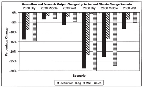
Figure 15. Streamflow and economic output changes by sector and climate change scenario.
Table 2. Estimated Changes in Direct Economic Output by Sector and by Climate Change Scenario
| Climate Change Scenario |
% Change in Average Annual Runoff |
Economic Sector millions of 2000 $ (percent of sector total) |
|||
| Agriculture | Municipal and Industrial |
Reservoir Recreation |
Total* | ||
| 2030 Dry | -13.7% | -33.8 (-8.9%) |
-1.3 (-0.1%) |
-3.0 (-14.7%) |
-38.1 (-2.0%) |
| 2030 Mid | -3.5% | -7.1 (-1.9%) |
-0.6 (-0.04%) |
-0.7 |
-8.4 (-0.4%) |
| 2030 Wet | -6.3% | -8.8 (-2.3%) |
-0.6 (-0.04%) |
-0.9 (-4.6%) |
-10.3 (-0.5) |
| 2080 Dry | -28.7% | -82.6 (-21.9%) |
-12.0 (-0.6%) |
-6.1 (-31.7%) |
-100.7 (-4.0%) |
| 2080 Mid | -22.8% | -50.9 (-13.5%) |
-5.5 (-0.3%) |
-5.3 (-27.3%) |
-61.7 (-2.4%) |
| 2080 Wet | -8.3% | -13.2 (-3.5%) |
0.0 (0%) |
-1.0 (-5.1%) |
-14.2 (-0.6%) |
| * In 2006, New Mexico’s total gross domestic product was estimated at $76 billion (NMBBER, 2006), and, therefore, even estimated direct losses greater than $100 million are less than 1/2 of 1% of the regional economic output. | |||||
For example, under the most extreme (2080 Dry), for example, average agricultural water use declines by 33% and results in an average economic reduction of $82.6 million (22%) compared to the population-adjusted 2080 baseline run; whereas water use in the urban sector falls less than 2%, with estimated economic losses of $12 million (0.6%) from a baseline value of $2.1 billion. Add to this estimated losses of $6.1 million for reservoir recreation, and total modeled economic losses under this severe scenario reach nearly $101 million (year 2000 dollars)—approximately 4% of the estimated total $2.5 billion in water-generated direct economic benefits.
Although direct economic losses to agricultural producers are potentially substantial by themselves, considerable economic consequences and disruption to related industries and employment levels are also possible—these are referred to as indirect and secondary effects.
Secondary Economic Effects. Secondary impacts take the form of “losses” in income or employment in agriculture-related industries and locations, and of “gains” in industries and locations to which water is transferred. For example, water that leaves agriculture and reduces irrigated acreage not only reduces farm incomes (the direct effect) but also reduces the demand for supporting economic services, including upstream activities such as farm machinery and repair, seed and chemical inputs, and labor, and downstream activities such as farm product processing and manufacturing. This can generate significant economic hardship and dislocation.
Although many economists consider secondary economic effect to be the result of economic restructuring that merely shifts or transfers economic activities—i.e., changes in the types or location of jobs with no measurable effect on overall economic performance and, therefore, of no net economic consequence— there are actually many reasons why these effects should not be readily dismissed. First, though population changes may propel water transfers to urban areas, with perhaps a shift in potential employment opportunities from the farm to the city, water transfers induced by climate change are fundamentally concerned with an absolute reduction in water supply, not simply with relocating an economic activity. Second, as Howe (1997) points out in describing inter-basin water transfers, there are likely to be severe and lasting economic repercussions to the regions water is leaving. People are not so easily uprooted and retrained. Substantial transition costs are likely in providing the needed “safety net” of support to rural economies that must adapt to reductions or loss of agriculture. Many rural communities in New Mexico include disadvantaged Native American and Hispanic communities that are likely to suffer disproportionately in attempting to adjust to the loss of income and lack of viable alternatives for economic development and employment.
Such secondary effects are difficult to measure and account for accurately. Most often, these effects are estimated as economic multipliers to the estimated direct effects. Hall and Skaggs (2003), for example, estimate an economic output multiplier of 1.61 for vegetable production in Southern New Mexico. In other words, for each $1 of vegetables produced, an additional $0.61 is contributed to the economy by upstream and downstream economic activities. Lillywhite et al. (2007a, 2007b) estimate multipliers for other agricultural industries ranging from 1.55 to 1.8. Allowing for a bit wider range in economic impacts and dislocation, e.g., a range in multiplier effects from 1.5 to 3, Table 3 shows estimated direct, indirect, and total economic effects of climate change on New Mexico’s water resources. These impacts range from a loss of between $15 million and $114 million in the 2030s to as much as $302 million in the 2080s under the relatively severe 2080 Dry scenario.
Table 3. Impact of Climate Change on the Direct and Secondary Economic Output of New Mexico
| Climate Change Scenario Runoff |
% Change in Average Annual (millions of 2000 $) |
Direct and Secondary Economics Impacts | ||
| Direct Impacts (millions of 2000 $) |
Secondary Impacts# (millions of 2000 $) |
Total Impacts* | ||
| 2030 Dry | -13.7% | -38.1 | -19.1 to -76.2 | -57.2 to -114.3 |
| 2030 Mid | -3.5% | -8.4 | -4.2 to -16.8 | -12.6 to -25.2 |
| 2030 Wet | -6.3% | -10.3 | -5.2 to -20.6 | -15.5 to -30.9 |
| 2080 Dry | -28.7% | -100.7 | -50.4 to -201.4 | -151.1 to -302.1 |
| 2080 Mid | -22.8% | -61.7 | -30.9 to -123.4 | -92.6 to -185.1 |
| 2080 Wet | -8.3% | -14.2 | -7.1 to -28.4 | -21.3 to -42.6 |
| # Secondary economic impacts are estimated at 0.5 to 2.0 times the direct impacts. This is arrived at by subtracting the direct impacts from estimates of total output impacts using a range of total output impact multipliers from 1.5 to 3.0 based on available studies and incorporating a margin of safety. For example, Hall and Skaggs (2003) estimate a total output impact multiplier of 1.61 for vegetable production in southern New Mexico; Lillywhite et al. (2007) estimate an impact multiplier of 1.55 for the New Mexico dairy industry and an estimate of 1.80 for the state’s pecan industry. * In 2006, New Mexico’s total gross domestic product was estimated at $76 billion (NMBBER, 2006), and, therefore, even estimated total economic losses greater than $300 million are less than 1% of the regional economic output. |
||||
Assumptions, Uncertainties, Omissions and Other Potential Biases
The presentation of the estimated potential economic consequences from climate change closes with a discussion and concern for the unaccounted-for effects that flow from model assumptions, uncertainties, and omissions. Here are highlighted—at least qualitatively—the nature of some significant additional concerns that condition the quantitative assessment. The following may not exhaust all the potential concerns, but does highlight key areas and limitations.
The costs of water transfers, respect for property rights, and the potential costs of conflict are not represented well at all. This is perhaps the most contentious and undervalued of all the omissions in the assessment. The modeling framework assumes neatly organized and efficiently functioning water markets in which buyers and sellers behave rationally and cooperatively with perfect information, foresight, and knowledge. In actuality, the potential for significant economic and legal conflict is not only real but likely unavoidable and very difficult to measure a priori. Absent a publicly and politically acceptable form of eminent domain and an accepted framework for compensable takings, there will likely be long, protracted litigation that will make water transfers from agriculture to municipal users anything but “frictionless” as the model assumes. Consider, for example, the tens of millions of dollars spent to date in attempting to accommodate stakeholder concerns in a “cooperative, consensus building exercise” to address the water problems of the San Francisco Bay-Delta in California. Without any promise of resolution—after more than twelve years of trying—the CALFED process is, like most western water issues, more and more likely to end up in litigation. Unresolved water rights issues flourish along the Rio Grande. Adjudication of water rights is long and contentious and not likely to be clearly resolved in the foreseeable future. Add to this the prior and paramount water rights reserved under the Winters Doctrine for the many tribes and pueblos of the Rio Grande region, and there are legal knots within knots that will add to water transfer costs—perhaps by many multiples.
Agriculture provides many valuable but uncompensated—and often unrecognized—services that will also be lost as water is transferred. Farms scattered throughout the Rio Grande region create green, open spaces enjoyed for their scenic beauty and by flocks of birds and other wildlife that migrate and traverse the arid rangelands of New Mexico in search of food, water, and refuge. Farming and agriculture are nature-based activities that are consistent with core public values such as stewardship of the land and water. Pastoral activities and landscapes are valuable for their ability to stimulate imagination, calm anxiety, restore connections to nature, and remind people of their long-enduring connection to the land and to the food it provides. Withering the agricultural lands of the Rio Grande will have unmeasured costs as land fragments into other uses or reverts to desert rangeland.
Adequacy and reliability of expected inter-basin transfers is called into question by recent studies and reports. For example, the 94,200 acre-feet of annual deliveries to the San Juan Chama system—accounting for 5% and 7.3% of native tributary inflow under current baseline and 2080 Dry scenarios, respectively—might rely on an overly optimistic estimate of available future flows (Christensen et al., 2006; NRC, 2007). After investing $275 million directly for its construction and making it a principal source of municipal water supply, the city of Albuquerque is particularly vulnerable to a reduction in this diversion. Making up for reductions in San Juan Chama water will exacerbate conflicts and costs associated with agricultural users and potentially with nearby pueblos and tribes.
The effects of increased flooding are not addressed and could be a very important and damaging feature of climate change. As the wet scenarios show, and as indicated by both other climate change research and recent experience, there is a measurable likelihood that summer precipitation associated with monsoonal flow and thunderstorm activity could increase across the Southwest, and in the Rio Grande basin in particular.9 The year 2006, for example, was the worst year in recent history for flooding and flood damages in the Southern Rio Grande of New Mexico and the El Paso, Texas region. The Rio Grande and some of its tributaries not only left their banks but breached levees in some areas, causing millions of dollars in flood damages in El Paso and near Hatch, New Mexico. Recent assessments by the Federal Emergency Management Agency (FEMA) indicate that aging levee and flood control infrastructure is degrading in the region and provides much less flood protection than previously indicated by 100-year floodplain maps. With increasing numbers of both people and economic assets at risk, climatic changes that increase the frequency and intensity of summer monsoonal storms in the Southwest are sure to exacerbate the severity and frequency of flood damages in the region.
Maintaining water quality is likely to be more difficult under climate change. Reduced streamflow lowers assimilative capacity for both point and non-point pollutants. In non-attainment reaches of the river lower TMDLs (total maximum daily load) might be expected and could raise control costs. Climate change might also lead some river reaches to fall out of attainment and require TMDLs and higher pollution control costs. Salinity is of particular concern in Southern New Mexico. Salinity concentrations continually rise as the Rio Grande journeys south, picking up loadings not only from urban wastewater and agricultural return flows but also from upwelling of salt-concentrated spring waters. With lower streamflow and runoff to dilute salinity, concentrations could be expected to rise. Currently, salinity is damaging only in the extreme southern part of the watershed, particularly near El Paso, where concentrations in excess of 2000 ppm are common. But without sufficient irrigation water to leach and resist the buildup of salts, salinity problems could become more common and severe for New Mexico water users in the future. For example, each acre of irrigated farmland in Southern New Mexico can expect to receive 2–3 tons of salt each year from surface irrigation water (presently containing concentrations between 500 ppm and 800 ppm). If salinity concentrations rise as a result of reduced flows, additional irrigation water for salt leaching would be needed to maintain agriculturally productive soils.
Climate change will affect New Mexico in significant ways beyond dewatering rivers and streams. Increased drying of soils and significant reductions in soil moisture are likely to occur as potential evapotranspiration rises with increasing temperatures (Wang, 2005).10 These effects will compound the adverse effects of changes in the hydrology of runoff and water availability throughout New Mexico. Such changes will affect the quality and condition of New Mexico’s forests and rangelands, which is likely to accelerate the severity and extent of forest fires and diminish forage production on rangelands, adversely impacting livestock and wildlife across the region (Hurd et al., 2007). Such changes in range productivity and livestock production due to climate change will likely add to the estimated agricultural sector impacts in New Mexico by damaging its most important agricultural activity, beef cattle, accounting for about 40% of agricultural income, or $2 billion in cash receipts (NMDA, 2005).
Additional impacts of climate change on New Mexico’s people and resources are found in two recent assessments of climate change.11 Watkins (2006) surveys the literature on climate change, hydrology, and water-related impacts and their potential inferences for New Mexico. Her findings are substantially consistent with those in this study; for example, she finds a consensus on the likelihood of rising temperatures and resulting hotter summers and milder winters. Regarding snowpack and snowmelt, she observes that snowpack would be less enduring under rising winter temperatures, leading to earlier snowmelt— pushing peak runoff ahead 4 to 6 weeks—and a relative shift from snow to rain. Furthermore, her findings confirm the likelihood of increased evaporation losses from streams, soils, and reservoirs, and of increased evapotranspiration. Finally, she finds support for increased likelihood of more frequent and severe extreme events—both floods and droughts.
Ecological and cultural impacts are uncounted in the assessment. Substantial changes in the natural hydrograph and intensification of managed uses will severely disrupt stream ecology and health, which may have additional implications for managing the endangered Rio Grande Silvery Minnow (Meyer, 1997). Additionally, long-standing Hispanic acequia communities will likely be early targets of water transfer—causing local economic dislocation and increased poverty (Rivera, 1996; Selcraig, 2002). Those communities that resist water transfers—either due to restrictions that the State Engineer might place on their water rights under New Mexico water statutes that require consideration of the public welfare when a water transfer is permitted (Bokum, 1991), or owing to a particularly powerful degree of cooperation among farmers—may also suffer as a result of a hydrographic shift. Because of a lack of storage infrastructure and vulnerable delivery systems, earlier and higher peak runoff could inundate acequia systems and fields early in the season and provide insufficient water during peak growing needs.
Additional related industries could also be negatively affected by climate changes and by the loss of agriculture and damage to ecosystem health and cultural resources. For example, tourism, arts, and recreation, which together contribute $360 million to New Mexico’s economy, might decline as the state’s unique landscapes, environment, and scenic opportunities are potentially degraded by changes in riparian ecosystems and agrarian land use (Rivera, 1996).
Each of these concerns taken individually adds considerably to the expected economic impacts from climate change. Taken together, there is sizable uncertainty in the extent to which economic damages, quality of life, ecosystem effects, and the overall severity of potential harm are unaccounted for by the model results. At least on a qualitative basis, there is significant cause for concern about the nature and magnitude of potential changes to New Mexico’s economy, landscape, and quality of life as a result of climatic change.
Findings and Conclusions
Ultimately, water is used by people, plants and animals—either directly consumed or indirectly used in growing food and providing economic and ecological services.
Under current climate there is virtually no spare water in New Mexico. Imagine a very plausible future, as this study attempts to, of significantly less water and at the same time significantly more people. Though improvements in water-use efficiency will be increasingly important to adopt and use—and will likely be further stimulated by economic prices that are allowed to signal increasing scarcity—this assessment puts light on the likely need to reorganize patterns of water use or else risk significant disruption in some of the important services provided by the state’s water resources.
A particular strength of the hydro-economic approach is its capacity to identify where and to what extent significant reorganizing of water uses will be potentially most rewarding from a watershed perspective. In this case, the results indicate the most expedient and least economically disruptive adaptation is to transfer water from agriculture as needed to maintain urban uses, growth, and economic development. In some ways these results highlight the obvious: a lot of water in New Mexico—87% or more if lawns, parks and golf courses are included—is consumed by plants. These are plants that provide food for people, for dairy cows, and for other livestock, but nonetheless plants; and the food they provide can almost surely be replaced by purchases from other places. Of course, if water transfers from agriculture are not as forthcoming as the hydro-economic model assumes, there could be significantly more economic dislocation in other sectors of the economy.
As described previously, agriculture’s real value—and the real loss to New Mexico’s residents, tourists, and wildlife—may not be so much in the market value of its agricultural produce but in the auxiliary services that agriculture provides to the environment and to quality of life. Losses and transfers—amounting to perhaps more than 30% of current water use levels—will dramatically and deleteriously affect agricultural systems, communities, and environments across the region. Therefore, in our view, such losses as must be accommodated should be regarded with both respect and regret, and fundamentally matched with an equal regard and effort to eliminate and guard against wasteful and capricious uses by urban and industrial water users. Absent this sentiment and action, rural communities, including farmers, pueblos, tribes, and acequias—along with their political allies and representatives—will most certainly fight to defend their way of life and their legal and constitutional rights to use and control water for their own benefit.
The following summarizes most of the key points developed in this assessment:
- Climate change scenarios result in less snowpack, earlier snow melt, and higher evaporative demands. The resulting change in runoff will affect vegetative cover in the watershed and habitat for various species.
- Substantial and transformational disruption to New Mexico’s agricultural and rural economy can be expected in the future as climate changes. Under the best economic and institutional assumptions, direct economic losses of up to $100 million are estimated, largely suffered in the agricultural sector under relatively severe climate changes by 2080, with an additional $200 million in indirect economic losses anticipated.
- These economic estimates almost surely understate the severity and extent of economic, social, and ecological disruption that is likely to result from moderate-to-severe changes in climate. For example, water transfers are likely to entail significant transactions costs because of unsettled water right issues, including protracted litigation, water right adjudication, and transfer approval procedures that must
protect against adverse effects on third-parties and the public welfare. - In addition, many sources of value that are potentially at risk under climate change have not been captured in the analysis. Examples of values that are not reflected include the expansive ecological and social services that agriculture provides, additional ecological and environmental services by flowing water in riparian systems, and further erosion and loss of cultural values and services from historical acequias and community irrigation systems.
The research findings suggest, particularly so when the limitations are given consideration, that New Mexico’s social, economic, and environmental systems are highly vulnerable to changes and disruptions to water supplies potentially caused by climate change. Thus, the need is highlighted for water users, communities, organizations, and institutions in New Mexico at every level and in every sector to begin considering possible adaptive strategies for making better use of their water resources.
Acknowledgements
This research was supported by a grant from the National Commission on Energy Policy, which made collaborations possible and provided the opportunity to work with such a gifted and talented group of researchers and academics. Of these we are especially grateful for the support and encouragement of Joel Smith of Stratus Consulting and Dr. Ken Strzepek of the University of Colorado. Special appreciation is extended to Dr. Coonrod’s graduate assistants Alandren Etlantus, Kelly Isaacson and Isaiah Pedro for their expertise in applying the WATBAL model. Thanks and appreciation is extended to Anne Watkins of the New Mexico Office of the State Engineer and to Dr. Dave Gutzler of the Earth & Planetary Sciences Department at the University of New Mexico for their work and contributions addressing potential climate change impacts on New Mexico’s water resources, and to Drs. Jim Booker of Siena College and Frank Ward of New Mexico State University, whose work Dr. Hurd proudly stands upon, for their efforts to carefully model the hydro-economy of the upper Rio Grande. Our appreciation is extended to Drs. Jay Lund of the University of California–Davis and Bonnie Colby of the University of Arizonia for their considerate and careful review of the final manuscript and their very helpful suggestions. Finally, Dr. Hurd would like to thank the leadership of the Agricultural Experiment Station of New Mexico State University for their ongoing support of his research program.
References
ATWG, Agency Technical Work Group (2005). Potential Effects of Climate Change on New Mexico. Santa Fe, NM: State of New Mexico.
Bokum, C. (1991). Implementing the Public Welfare Requirement in New Mexico’s Water Code. Albuquerque, NM: Western Governor’s Association and Western States Water Council.
Booker, J. F. & Young, R. A. (1994). Modeling Intrastate and Interstate Markets for Colorado River Water Resources. Journal of Environmental Economics and Management, 26, 66-87.
Booker, J. F. & Young Robert A. (1991). Economic Impacts of Alternative Water Allocation Institutions in the Colorado River Basin (Rep. No. 161).
Brooke, A., Kendrick, D., & Meeraus, A. (1988). GAMS: A User’s Guide. San Francisco, CA: The Scientific Press.
Cai, X. M., McKinney, D. C., & Lasdon, L. S. (2003). Integrated hydrologic-agronomic-economic model for river basin management. Journal of Water Resources Planning and Management, 129, 4-17.
Christensen, N. S., Wood, A. W., Voisin, N., Lettenmaier, D. P., & Palmer, R. N. (2004). The effects of climate change on the hydrology and water resources of the Colorado River basin. Climatic Change, 62, 337-363.
Doggett, M., Daly, C., Smith, J., Gibson, W., Taylor, G., Johnson, G. et al. (2004). High-resolution 1971–2000 mean monthly temperature maps for the western United States. In 14th Conference on Applied Climatology (Paper 4.3, CD-ROM). American Meteorological Society (AMS).
Draper, A. J., Jenkins, M. W., Kirby, K. W., Lund, J. R., & Howitt, R. E. (2003). Economic-engineering optimization for California water management. Journal of Water Resources Planning and Management, 129, 155-164.
FAO (1992). Expert consultations on revision of FAO methodologies for crop water requirements. Rome: Food and Agriculture Organisation of the United Nations, Land and Water Development Division.
Hall, T. Y. & Skaggs, R. K. (2003). Economic Impact of Southern New Mexico Vegetable Production and Processing (Rep. No. 9). Las Cruces: New Mexico State University, Chile Task Force.
Howe, C. W. (1997). Increasing Efficiency in Water Markets: Examples from the Western United States. In T.L.Anderson & P. J. Hill (Eds.), Water Marketing—the Next Generation (pp. 79-100). New York: Rowman and Littlefield Publishers.
Hurd, B. H. (2006). Water conservation and residential landscapes: Household preferences, household choices. Journal of Agricultural and Resource Economics, 31, 173-192.
Hurd, B. H., Brown, C., Greenlee, J., Grandados, A., & Hendrie, M. (2006). Assessing Water Resource Vulnerability for Arid Watersheds: GIS-based Research in the Paso del Norte Region. New Mexico Journal of Science, 44, 39-61.
Hurd, B. H., Callaway, J. M., Smith, J. B., & Kirshen, P. (1999). Economic Effects of Climate Change on U.S. Water Resources. In R. Mendelsohn & J. Neumann (Eds.), The Impact of Climate Change on the United States Economy (pp. 133-177). Cambride, UK: Cambridge University Press.
Hurd, B. H., Callaway, M., Smith, J., & Kirshen, P. (2004). Climatic change and U.S. water resources: From modeled watershed impacts to national estimates. Journal of the American Water Resources
Association, 40, 129-148.
Hurd, B. H. & Harrod, M. (2001). Water Resources: Economic Analysis. In R.Mendelsohn (Ed.), Global Warming and the American Economy: A Regional Assessment of Climate Change Impacts (pp. 106-131). Northhampton, MA: Edward Elgar Publishing.
Hurd, B. H., Leary, N., Jones, R., & Smith, J. (1999). Relative regional vulnerability of water resources to climate change. Journal of the American Water Resources Association, 35, 1399-1409.
Hurd, B. H., Torell, L. A., & McDaniel, K. C. (2007). Perspectives on Rangeland Management: Stocking Rates, Seasonal Forecasts, and the Value of Weather Information to New Mexico Ranchers (Research Report 759). Las Cruces: New Mexico State University, Agricultural Experiment Station.
IPCC, Intergovernmental Panel on Climate Change, Working Group I (2007). Climate Change 2007: The Physical Science Basis, Summary For Policymakers. Geneva, Switzerland: IPCC.
Jenkins, M. W., Lund, J. R., Howitt, R. E., Draper, A. J., Msangi, S. M., Tanaka, S. K. et al. (2004). Optimization of California’s water supply system: Results and insights. Journal of Water Resources Planning and Management, 130, 271-280.
JWRPM. (2006). Special Issue: Economic-Engineering Analysis of Water Resource Systems. Journal of Water Resources Planning and Management, 132[6], 399-512.
Lillywhite, J. M., Crawford, T., Libbin, J., & Peach, J. (2007). New Mexico’s Pecan Industry: Estimated Impacts on the State’s Economy (Bulletin 791). Las Cruces: New Mexico State University, Agricultural Experiment Station.
Lillywhite, J. M., Sullivan, H., Crawford, T., & Ashcroft, N. (2007). New Mexico Milk Production: Estimated Impacts on the State’s Economy (Bulletin 790). Las Cruces: New Mexico State University, Agricultural Experiment Station.
Malone, E. L., Smith, J. B., Brenkert, A. L., Hurd, B. H., Moss, R. H., & Bouille, D. (2004). Developing Socioeconomic Scenarios: For Use in Vulnerability and Adaptation Assessments, 9. New York: United Nations Development Program (UNDP), Global Environment Facility.
Meyer, J. (1997). Stream Health: Incorporating the Human Dimension to Advance Stream Ecology. Journal of the North American Benthological Society, 16, 439-447.
Nakicenovic, N. & Swart, R. (Eds.). (2000). Special Report on Emissions Scenarios: A Special Report of Working Group III of the Intergovernmental Panel on Climate Change. Cambridge, UK: Cambridge University Press.
NM BBER (2004). Projected Annual Population Growth Rates: New Mexico Counties. Albuquerque: Bureau of Business and Economic Research, University of New Mexico.
NM BBER (2006). Real New Mexico Gross Domestic Product by Industry. http://www.unm.edu/~bber/economy.htm.
NMDA (2005). New Mexico Agricultural Statistics, 2004. Las Cruces: New Mexico Department of Agriculture.
Nohara, D., Kitoh, A., Hosaka, M., & Oki, T. (2006). Impact of climate change on river discharge projected by multimodel ensemble. Journal of Hydrometeorology, 7, 1076-1089.
NRC (2007). Colorado River Basin Water Management: Evaluating and Adjusting to Hydroclimatic Variability. Washington, D.C.: National Academies Press.
Null, S. E. & Lund, J. R. (2006). Reassembling Hetch Hetchy: Water Supply Without O’Shaughnessy Dam. Journal of the American Water Resources Association, 42, 395-408.
Plog, S. (1997). Ancient Peoples of the American Southwest. London: Thames and Hudson.
Rivera, J. A. (1996). Irrigation Communities of the Upper Rio Grande Bioregion: Sustainable Resource Use in the Global Context. Natural Resources Journal, 36, 491-520.
Selcraig, B. (2002). Digging Ditches: Narrow, Humble Irrigation Ditches Called Acequias Sustain an Endangered Way of Life. Smithsonian, 32, 54-63.
Smith, J. B. & Wagner, C. (2006). Scenarios for the National Commission on Energy Policy. Boulder, CO.
Tanaka, S. K., Zhu, T. J., Lund, J. R., Howitt, R. E., Jenkins, M. W., Pulido, M. A. et al. (2006). Climate warming and water management adaptation for California. Climatic Change, 76, 361-387.
Vaux, H. J. Jr. & Howitt, R. E. (1984). Managing Water Scarcity: An Evaluation of Interregional Transfers. Water Resources Research, 20, 785-792.
Wang, G. L. (2005). Agricultural drought in a future climate: results from 15 global climate models participating in the IPCC 4th assessment. Climate Dynamics, 25, 739-753.
Ward, F. A., Hurd, B. H., Rahmani, T., & Gollehon, N. (2006). Economic impacts of federal policy responses to drought in the Rio Grande Basin. Water Resources Research, 42, W03420.
Ward, F. A., Young, R., Lacewell, R., King, J. P., Frasier, M., McGuckin, J. T. et al. (2001). Institutional Adjustments for Coping with Prolonged and Severe Drought in the Rio Grande Basin. Las Cruces: New Mexico Water Resources Research Institute.
Watkins, A. (2006). The Impact of Climate Change on New Mexico’s Water Supply and Ability to Manage Water Resources. Santa Fe: New Mexico Office of the State Engineer.
Woodhouse, C. A., et al. (2004). TreeFlow Colorado Streamflow Reconstructions. IGBP PAGES/World Data Center for Paleoclimatology Data Contribution Series # 2004-029. NOAA/NGDC Paleoclimatology Program, Boulder CO, USA.
Yates, D. (1996). WATBAL: An Integrated Water Balance Model for Climate Impact Assessment of River Basin Runoff. Water Resources Development, 12, 121-139.
Yates, D. & Strzepek, K. (1994). Comparison of models for climate change assessment of river basin runoff (Rep. No. WP-94-46). Laxenburg, Austria: (IIASA) International Institute for Applied Systems Analysis.
Yates, D. N. (1997). Approaches to continental scale runoff for integrated assessment models. Journal of Hydrology, 201, 289-310.
1 A growing consensus among anthropologists attributes the regional collapse of indigenous settlements prior to European arrival to multiple factors importantly including climatic extremes (Plog, 1997). Peoples such as the Anasazi, Hohokam and Mogollon abandoned long-held settlements during a period that tree-ring analysis has identified as the “Great Drought” at the end of the 13th century.
2 The Intergovernmental Panel on Climate Change (IPCC) published a Special Report on Emissions Scenarios (SRES, Nakicenovic et al., 2000), which consisted of four families of emissions scenarios that ranged from very low population and very high economic growth (A1) to very high population and somewhat low economic growth (A2) to somewhat low economic growth and moderate population (B2) to moderate economic growth and low population (B1). Of these, the A1B scenario comes closest to U.S. government projections for population and income growth and to the “business as usual” emissions projection, known as IS92a. Note, however, that the A1B scenario also has the highest emissions of sulfate aerosols of all the SRES scenarios, with a peak in 2030 and rapid decline thereafter.
3 In addition to the limitations and assumptions previously discussed, the RGHE model uses a simplified representation of groundwater and aquifer storage and its connectivity to surface water systems. For example, Albuquerque currently relies on groundwater for its public water supply system. However, the hydrologic connectivity of surface- and ground-water systems is well recognized, including the requirement that future groundwater development be offset by retirement of surface water rights. The model assumes that over the long run water use is constrained by available surface water supplies. To implement this perspective, the model assumes that groundwater and aquifer use must be offset such that by the terminal model time period (i.e., after 30 years) aquifer volumes are returned to their initial storage volumes.
4 Exception is made for the managed transfers from the Closed Basin Project (CBP) and from the San Juan Chama (SJC) trans-basin diversion. For the CBP and SJC, annual deliveries of 21 kaf/yr and 94.2 kaf/yr are assumed (the latter is based on average importations since 1970; however, 110 kaf/yr is authorized). Imported water is distributed across months in approximate proportion to system water demands. Furthermore, imports are assumed not to vary with climate change. According to recent research on the effects of climate change on the Colorado River (NRC, 2007; Christensen et al., 2004)—the source of the SJC water—it may be a strong assumption that this amount of water will be available in the event of significant climate change. The potential reduction or loss of this water will have a significant impact on Albuquerque water users.
5 This stands in contrast to earlier studies (e.g., Hurd et al., 1999) where the modeled shift in agricultural demand resulted in an expansion of so-called producers’ surplus. Here, the value of agricultural production is maintained on the condition that the necessary water is supplied to meet the change in irrigation requirements. As water is then reduced, so is the generated economic value. It is also assumed that relative agricultural prices are NOT affected by climate changes—a strong assumption that depends on sector-wide market effects that are beyond the present scope of analysis.
6See Hurd (2006) for discussion of current trends in New Mexico residential landscapes.
7 The slopes of the curves in Figure 12 are relatively constant. This constancy reflects the assumed absence of changes in streamflow variability, and the primary focus of the present analysis on changes in average conditions. There is quite significant natural variability in the Rio Grande watershed, variability that is captured in the current analysis. Climate change, however, could change runoff variability and, if increased, further exacerbate the relative likelihood of drought and/or flood events. Changes that increase runoff variability would result, for example, in a relative flattening of the scenario curves shown in Figure 12.
8 Implicit model prices are the marginal values that are estimated by observing the “shadow price” on water supply constraints in the model. Though these “values” are illustrative of the relative values under different population and water supply conditions, they are not necessarily indicative of actual market prices, which are a complex function of many factors affecting local water demand and water supply conditions, including speculative development. These estimated values are most reflective of the marginal value of water in agriculture and not indicative of the willingness to pay for water of, for example, municipal and industrial water users.
9 Nohara et al. (2006) examine the effects of climate change using 19 GCMs simulating the SRES A1B scenarios (just as in this study) on the hydrology and river discharge of 24 of the world’s most important river basins, including the entire Rio Grande system. Results for the Rio Grande show wide divergence in seasonal runoff across the GCMs, with several showing pronounced summer runoff that is most closely associated with intense summer storms and the likelihood of regional flash floods.
10 Wang (2005) examines changes in soil moisture conditions across 15 GCMs and finds substantial consistency across the models in projecting significant reductions in soil moisture in all seasons for the southwestern United States.
11 These assessments were initiated under Governor Richardson’s Climate Change and Greenhouse Gas Reduction Executive Order (05-033) and were conducted by New Mexico’s Office of the State Engineer on potential impacts on the water resources (Watkins, 2006) and by the New Mexico Environment Department (ATWG, 2005).
To find more resources for your business, home, or family, visit the College of Agriculture and Home Economics on the World Wide Web at aces.nmsu.edu.
Contents of publications may be freely reproduced for educational purposes. All other rights reserved. For permission to use publications for other purposes, contact pubs@nmsu.edu or the authors listed on the publication.
New Mexico State University is an equal opportunity/affirmative action employer and educator. NMSU and the U.S. Department of Agriculture cooperating.
Printed and electronically distributed August 2008, Las Cruces, NM.
