Research Report 779
L. Allen Torell, Brent Dixon, Dan McCullom
College of Agricultural, Consumer and Environmental Sciences, New Mexico State University (Print Friendly PDF)
Authors: Respectively, Professor, Department of Agricultural Economics and Agricultural Business, New Mexico State University; Graduate Research Assistant, Department of Agricultural Economics and Agricultural Business, NMSU; and Economist, U.S. Forest Service Rocky Mountain Research Station.
Table of Contents
Introduction
Hedonic Pricing Models
Recent Trends in Agricultural Land Values
Methods
Results
Discussion
Acknowledgements
Literature Cited
Appendix A: Estimation Issues For Hedonic Ranch Value Models
Appendix B: Using Ranval2010
Introduction
The objectives of this study were to describe recent trends in the market value of New Mexico ranches and grazing permits and to explore the key factors that influence the value of New Mexico ranches using a hedonic pricing model. The study updates a long history of New Mexico ranch value studies. These earlier studies provided hedonic models that could be used to estimate the value of particular ranches of interest (Torell et al., 2000; Torell et al., 2003), and this study updates the RANVAL model (Torell, 2011). The hedonic regression models were estimated from statistical analyses of ranch sales data provided by Farm Credit Services (FCS) of New Mexico. The model was used to estimate the trend in value for ranches in different areas of the state and with differing amounts of leased public and state trust land included. We first review the history of ranch value studies done in New Mexico and in other states and review what is known about the changing motives for ranch purchase. The data and hedonic models for this most recent analysis are then described.
Hedonic Pricing Models
Hedonic models use regression analysis to decompose the price of an item into separate components that determine price (Taylor, 2003). The real estate market is a common example of an application of a hedonic pricing model. In this application, the hedonic property model begins with a consumer who derives satisfaction from real estate ownership and from other goods (Taylor, 2003). Grazing lands and other business properties also have future income earning potential that creates purchase incentive. Thus, the willingness to pay for a real estate property is determined by income earning potential, development potential, and amenity characteristics. A sample of real estate transactions is gathered, and regression analysis is used to relate selling price to the key characteristics believed to influence price. Appraisal methodology treats the hedonic regression as essentially a robust form of the sales comparison approach (Kilpatrick, 2004). Hedonic models are commonly used in tax assessment, product pricing, academic studies, and mass appraisal projects (Taylor, 2003).
Ranchland Hedonic Models and Motives for Ranch Purchase
When agricultural land is viewed solely for its income earning potential, a present value model describes the maximum value justifiably paid for the land asset (Burt, 1986). Because livestock production and profit were the traditional motivations for ranch purchase, factors that influence income earning potential, like rangeland productivity, forage availability, and expected production costs, were the primary factors explaining ranchland price differences in early hedonic ranch valuation models. This included studies in Arizona (Martin and Jefferies, 1966), Utah (Workman and King, 1982), Oregon (Winter and Whittaker, 1981), New Mexico (Torell and Fowler, 1986), and Wyoming (Collins, 1983; Sunderman and Spahr, 1994; Sunderman et al., 2000). Yet, as early as the 1960s, some began to question livestock production and the profit motive as the only reasons for ranch purchase (Martin, 1966; Martin and Jefferies, 1966). At the time, deeded rangelands were estimated to be overpriced by nearly three times relative to the value justified for livestock production (Smith and Martin, 1972). Expectation of real appreciation of the real estate investment was a reason commonly given to explain the apparent price discrepancy (Martin and Jefferies, 1966; Melichar, 1979; Sunderman et al., 2000). Madsen et al. (1982) found that in 1980, productive ranch values based on income capitalization were generally consistent with observed market prices when agricultural uses predominated and land appreciation was factored in. Over time, there has been an increasing realization that ranchland values, including the value of federal and state grazing permits, are influenced by many factors not related to livestock production. The desired rural lifestyle and agrarian values described by Martin have significantly inflated the market value of both farms and ranches (Doye and Brorsen, 2011). Corresponding to this, more recent hedonic agricultural land valuation models have emphasized amenity values like scenic views and recreational opportunities on the property (Rimbey et al., 2007; Bergstrom and Ready, 2009).
By the early 2000s, Western ranches were described in the popular press as having become “pearls of great value” (Sands, 1998; Henderson, 2000). Scenic ranches with privacy and fishing and hunting opportunities had soared in value. The price of these recreation parcels had little to do with the value of the grass or livestock that might be produced. Gosnell et al. (2007) found that many ranch purchases in Wyoming and Montana were driven by the specific goal of obtaining exclusive access to fisheries. This was reflected in the Wyoming hedonic ranch value models estimated by Bastian et al. (2002a) and Wasson et al. (2010), where explanatory variables measuring hunting and fishing opportunities were highly significant determinants of ranchland value. Provision of wildlife habitat and access to a blue ribbon trout stream were also found to be important determinants of ranch sale prices for Montana ranches (Baird, 2010). Similarly, Torell et al. (2005) found hunting income and opportunities were major factors influencing the market value of New Mexico ranches. Income from wildlife added nearly 2.5 times more to ranch value than did livestock income. Sales brochures for Western ranches now emphasize recreational opportunities, scenic views, and lifestyle attributes (see for example http://fayranches.com and http://www.nm-ranches.com). People now buy ranches for personal reasons beyond just agricultural production. Land is real. You can visit it, walk on it, and enjoy it. Investors like the sense of place that comes from owning land in the country. They value the recreational opportunities provided and are willing to pay premium prices for ranches providing open space, rural living, agrarian values, and recreational opportunities.
Recent ranch buyers are more likely to be lifestyle seekers than professional profit-motivated ranchers. A West-wide survey of 1,052 public land ranchers found an approximate equal split between ranchers that depended heavily on the ranch for annual income versus those whose income came mostly from other sources (Gentner and Tanaka, 2002). Over the 1990 to 2001 period, Gosnell et al. (2006) found a shift in ranch ownership patterns around Yellowstone National Park from traditional ranchers (typically full-time livestock producers) to a more diverse group that included absentee owners focused on amenity and conservation values instead of livestock production. Locational differences exist, however. Gosnell and Travis (2005) found amenity buyers to make up only 15% of ranch buyers in rural Carbon County, MT, but over 60% of ranch purchases in Routt County, CO and Sublette County, WY (with close proximity to Steamboat Springs, CO and Jackson, WY, respectively) were amenity motivated.
New Mexico Hedonic Ranch Models
Table 1 shows key explanatory variables included in earlier hedonic ranch value models developed for New Mexico. Appendix A provides additional discussion about some of the key issues for estimating these hedonic models. This includes concern about how the dependent variable should be defined given the changing motivations for ranch purchase, inclusion of public and state lands on Western ranches, recognition that the land value estimate should not be negative, and correction for spatial autocorrelation between ranch sales.
Table 1. Previous New Mexico Ranch Value Studies
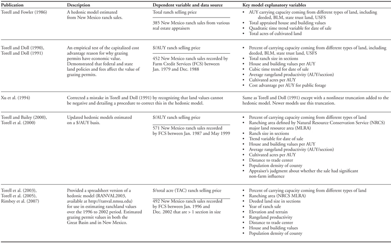
The first New Mexico hedonic model (Torell and Fowler, 1986) was a relatively simple model published shortly after the “farm crisis” of the early 1980s when farmland values declined for the first time since World War II. The total selling price of a ranch was estimated to be a quadratic function of date of sale with other explanatory variables, including the number of AUY1 leased from public (Bureau of Land Management [BLM] and U.S. Forest Service [USFS]) and state land, the grazing capacity of deeded lands, the appraised value of houses and buildings, the average rangeland productivity, and the number of cultivated acres. In general, as New Mexico models were expanded and improved, they indicated that ranch sale prices were dependent on rangeland productivity, income earning potential, ranching area, distance to a trade center, elevation, and the amount of leased land included with the sale. The amount of public and state land has proven to be one of the most important factors influencing the value of New Mexico ranches. There is a significant discount in price (relative to deeded land) when public and state trust lands are included with the sale. Grazing permit value is represented as an inflated price paid to the seller for the base property and/or livestock (Gardner, 1997; Egan and Watts, 1998). Though discounted in price, there is still a substantial economic value for grazing permits when transferred with the ranch sale. The ranch real estate market recognizes this permit value, even though legal compensation for the value of the grazing permit is limited if it is cancelled in whole or in part for other multiple use considerations (Grazing Leases and Permits, 2010).
Recent Trends in Agricultural Land Values
Real estate values greatly appreciated during the early to mid-2000s, as noted in a Time Magazine article released right before the housing market crash of 2006 (Poniewozik, 2005). Housing markets are once again in the news, but the focus now is on the dire straits and economic losses many homeowners experienced following the collapse of the home real estate market and subsequent economic downturn.
Unlike the housing market, agricultural land values have remained strong. Midwest farmland values have increased at rates not seen since the 1970s (Duffy, 2011). These increases are being driven by strong agricultural commodity demand and income, low interest rates, and a lack of alternative high-yield investments (AAEA, 2011; Messick, 2011). For the Western states, AAEA (2011) reported that agricultural land values peaked in 2008 with declines in 2009, but by 2011 were back to or slightly above 2008 peak values. The typical buyer in the recent market is an existing agricultural producer expanding an operation. AAEA (2011) noted a decrease in demand for rural residential, commercial, and recreational land.
Average New Mexico pasture values as reported by USDA-NASS (various issues) rose sharply over the 2004 to 2006 period, followed by declines in value during 2006 to 2007 (Figure 1). Reported cash rents for pasture in New Mexico increased over the 2005 to 2008 period, but not as much as land values, and thus rent-to-value ratios declined (Figure 1)2. Current USDA estimates of deeded pasture values in New Mexico are about $300/acre, with a cash rental rate of about $2.40/acre. Similar trends in pasture value and declines in rent-to-value ratios were reported for other intermountain states (USDA-NASS, various issues).

Figure 1. Average deeded pasture values reported by USDA in New Mexico, 1997 to 2011.
Several ranch appraisal firms have provided information and professional opinions and observations about recent trends in Western pasture and rangeland values. As noted by Greg Fay of Fay Ranches, a major brokerage and ranch management services business in Montana, Idaho, Wyoming, Colorado, and Oregon, very few ranches change hands relative to the residential market, and an exact percentage change in the market is hard to define. He notes a slowdown in the ranch real estate market starting in about 2006 to 2007, but also notes that recreational ranches with the highest-quality amenities have seen very little, if any, decline in value (Fay, 2011). He also notes a significant improvement in values from 2009 to 2010 and the first quarter of 2011. Norman Wheeler, a Montana ranch appraiser, gives a similar opinion of value trends (Wheeler, 2011). He notes that the ranch real estate market has split into various submarkets, with values based on location characteristics and the highest and best use of the ranch property. He categorizes one type of ranch as agricultural production-based and notes minimal increases in value over the 1996 to 2009 period, but also with minimal declines in value. He notes that these agricultural production-based ranches, along with high-amenity recreational ranches, are scarce and have maintained value. According to Wheeler, ranches with desirable amenities have continued to increase in value at a much faster rate than production-based ranches. Wheeler notes that the ranches that lost significant value after the real estate crash of 2006 were those with an anticipated but unrealized transition to a more valuable use for development or recreation. These over-listed properties are now selling in the markets appropriately reflecting their highest and best use (Wheeler, 2011).
Methods
Torell et al. (2005) used New Mexico ranch sales data collected from Farm Credit Services (FCS) for the years 1996 to 2002 to develop a New Mexico hedonic model. New FCS data3 were collected and combined with the earlier data set, and this updated analysis includes sales negotiated between January 1996 and April 2011. The three 2011 sales were treated as if they occurred in December 2010 in the statistical analysis.
Farm Credit Services appraisal data sheets contain extensive information about the documented sale, including financial terms of the sale; ranch location; acreage and livestock carrying capacity by type of land; the value of real property such as houses, buildings, and major structural improvements; and FCS appraiser estimates of income earning potential. The income appraisal sheet includes estimates of annual crop and livestock income, wildlife income, potential rental income of facilities and housing, and occasionally income from surface minerals like sand, gravel, and caliche. All comparable sales located and documented by FCS appraisers were included regardless of FCS loan involvement with the sale.
Some screening of sales in the analysis was used. First, the total size of the parcel purchased had to be >3,400 acres (>5 sections). This was an arbitrary size cutoff recognizing that the motivation of small parcel purchasers is highly variable. Properties with primarily irrigated cropland, irrigated pasture, or dry cropland (parcels with >50% cropland acreage) were excluded. Ranches where the stated purchase motivation was to develop a subdivision or multiple small tract home sites were excluded. Five additional sales, primarily located in north-central New Mexico, sold for over $5,000/acre and were also excluded. Initial attempts to include these sales in the hedonic model indicated a great deal of unexplained price variation, and these sales were considered outliers relative to other observed sales. These outliers fit into the high-amenity recreational ranch submarket described by Wheeler (2011).
The final sample included 659 ranch sales, and the locations of those sales are shown in Figure 2, overlaid over the major land resource areas (MLRA) defined by the USDA Natural Resources Conservation Service (NRCS)4. The NRCS MLRA designations are generally defined based on soil and vegetation characteristics (USDA-NRCS, 2006). These areas also vary in rangeland productivity, elevation, topography, and land ownership patterns. Ranch sales were included for all areas of the state except White Sands Missile Range in central New Mexico and Indian reservations in northwest New Mexico. Of the 659 total sales, 111 comprised entirely deeded land (16.8%). State land acres were included on 471 (71%) of the ranches, BLM on 302 ranches (46%), and USFS on 44 ranches (6.7%).
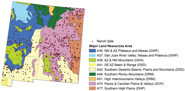
Figure 2. Ranch sale locations.
Characteristics, such as elevation of the ranch at the headquarters, distance to a paved road, and distance to the nearest trade center (Table 2), were defined from the township-range-section ranch location defined on the FCS appraisal sheets (usually the ranch headquarters location). Following the procedure of Torell et al. (2005), trade centers were considered to be cities large enough to support major shopping and cultural activities. Road distances from the ranch to a paved road and to the nearest trade center were calculated using the Google Maps website (Google, 2011).
Table 2. Defined Trade Centers
| El Paso, TX | Hobbs | Española | Lordsburg |
| Albuquerque | Carlsbad | Ruidoso | Santa Rosa |
| Las Cruces | Gallup | Grants | Clayton |
| Santa Fe | Deming | Socorro | |
| Roswell | Las Vegas | Truth or Consequences | |
| Farmington | Artesia | Raton | |
| Alamogordo | Silver City | Tucumcari | |
| Clovis | Lovington | Taos |
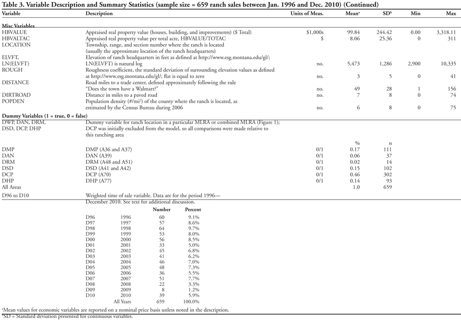
Table 3 provides a detailed listing of variables and a description of how variables were defined and computed, along with overall statistics from the ranch sales data. Following the procedures of FCS appraisers to estimate ranch income earning potential, we used the standard income appraisal approach based on forage lease value (Appraisal Institute and ASFMRA, 2000) with the following exceptions. Whereas FCS generally valued grazing capacity at about the USDA 11-Western-state average $/AUM lease rate, in our research forage value was recomputed at 70% of the USDA lease rate paid during the year of the ranch sale, assuming forage value is 70% of the reported value as reported by Bartlett et al. (2002) as a finding in several forage valuation studies. USDA 11-state lease rates gradually increased from about $10/AUM in 1996 to $15/AUM in 2010 (USDA-NASS, 2012).
Table 3. Variable Description and Summary Statistics (sample size = 659 ranch sales between Jan. 1996 and Dec. 2010)
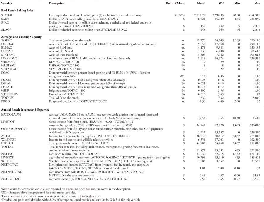
We recomputed the maintenance and management charge at 5% in all cases. The FCS-estimated wildlife income, crop income, rental income, and improvement valuation were used without modification. For consistency and accuracy, grazing fee payments were recalculated using fee rates paid during the year of the ranch sale. The income variables used in the regression analysis and in summary statistics were computed as net income coming from wildlife enterprises, with all other income grouped together as non-wildlife income. The income that was grouped was primarily from livestock production, but included a few sales that had headquarters rental income, mineral sales, Conservation Reserve Program (CRP) payments, and crop production. Ranch expenses were allocated based on the percentage of gross income included in the wildlife and non-wildlife categories. Ranch expenses primarily included grazing fees and management and maintenance charges.
Including wildlife income in the analysis was possible because New Mexico has a program whereby wildlife hunting permits are issued to landowners as compensation for providing wildlife habitat on private lands. Landowners have the option of using the wildlife permits themselves or selling them. Estimates of allowed wildlife harvest on each ranch were determined using a database of landowners with elk (rule 19.30.5) and antelope (rule 19.31.15) hunting authorizations as maintained by the New Mexico Department of Game and Fish (2004). Estimates of wildlife income for game species not in the Game and Fish database were also made by FCS appraisers based on conversations with landowners.
The annual market value of the wildlife permits was made by FCS appraisers from observed market conditions at the time the sale was recorded. Nominal market values assigned for bull elk permits were generally around $2,200 each in 2003 and 2004, increasing to $3,000 after 2005. Cow elk permits were valued at about $300 each. Buck deer permit values ranged from about $800 during the early years of the analysis to as high as $2,500. Assigned values for buck antelope ranged from about $750 in 2003 to double that by 2007. Not all appraisers consistently entered wildlife income on the appraisal sheet, and this is a data limitation.
In order to spatially visualize differences in ranch characteristics, we computed and categorized ranch sales statistics on a $/AUY, $/deeded acre ($/DAC), and $/total acre ($/TAC) basis. The distinction between deeded and total acres is that the total acre calculation includes all acres, including lands leased from federal and state land agencies (see Appendix A for additional discussion). Arc GIS 9 was used to spatially visualize regional differences in key variables, including percent leased land, non-wildlife income, wildlife income, and $/TAC, $/DAC, and $/AUY ranch sale prices. Each ranch sale is visualized as a dot based on the township, range, and section location of the ranch headquarters. The size of the data point indicates the ranch’s relative value.
Hedonic Model Estimation
The nominal-price hedonic model estimated in this report updates the similar truncated model estimated by Torell et al. (2005).5 We refer the interested reader to the earlier paper for a detailed description of the model, which is estimated on a $/TAC basis. Potential explanatory variables for the updated model are defined in Table 3. One new variable not considered in the earlier study, distance to a dirt road, was added as a potential explanatory variable. Statistically insignificant variables (P < 0.10) were not included in the final model unless there was strong theoretical justification for inclusion. For the final model, g(X,β) was defined to be:
g(X,β) = β1 + β2 NETAGTAC + β3 NETWILDTAC + β4 HBVALTAC + β5 LN(DEEDSECT) + β6 LN(ELVFT) + β7 DISTANCE + β8 POPDEN + β9 DSD + β10 DRM + β11 D98 + β12 D99 + β13 D00 + β14 D01 + β15 D02 + β16 D03 + β17 D04 + β18 D05 + β19 D06 + β20 D07 + β21 D08 + β22 D09 + β23 D10 + β24 D11 + β25 %STATEAC + β26 %USFSAC + β27 %BLMAC + β28 DUSFSAC + β29 DBLMAC + β30 DSTATEAC + β31 %IRR + β32 %DRYFARM (Equation 1)
The betas (βs) are estimated parameters. A truncation parameter (τ) is an additional estimated parameter, assuming normality of the errors (equation 5 in Torell et al., 2005). The model was estimated using nonlinear ordinary least squares (OLS) routines in SAS (PROC MODEL).
Dummy variables were included in the model for different MLRA areas as well as year of sale. For the ranching area dummy variables, the Central Plains area (DCP) was initially excluded from the model such that other area dummy variables (DWP, DAN, DRM, DSD, DHP) measured value relative to this area. As shown at the bottom of Table 3, 46% of the sales were located in the Central Plains MLRA (DCP = 1).
Time of sale was incorporated into the regression models with the dummy variable procedure used by Torell et al. (2005) and Sunderman et al. (2000). By this non-standard dummy variable definition, the value of the dummy variable for the year of sale is computed as the proportion of the year that remains after the sale date, while the dummy variable for the following year is one minus that proportion. The dummy variables for all other years are set to zero. As noted by Sunderman et al. (2000), this approach allows the rate of change in ranch values to be different through time and provides for a sale price continuum rather than an annual step function. All sales were defined to occur between January 1, 1996, and December 31, 2010.
Two different discounts are included in the final model for state and public lands. First, following Torell et al. (2005), the percentages of the purchased land acreage composed of state grazing leases, BLM leases, and USFS leases were explanatory variables in the model. Parameter estimates for β25, β26, and β27 (Equation 1) are expected to be negative and reflect a discount relative to deeded land when the percentage of land on leased areas increases by 1%.6 Similar to the earlier model of Torell et al. (2005), residual plots indicated the model tended to over-predict the market value of ranches that were almost entirely public and/or state land. Dummy variables were added to shift the intercept when over 90% of the ranch acreage was on public and state lands. Separate dummy variables were added for each land type so the discount for high-acreage permit ranches is not restricted to be the same. Other functional forms for the public land price discount were explored, but the linear definition with the added dummy variables provided the best fit.
Results
Ranch Sale Statistics
Summary statistics for the 659 study ranches are given on a $/TAC, $/AUY, and $/DAC basis in Tables 4, 5, and 6, respectively. Price statistics are presented on a nominal price basis. At the bottom of each table is a figure showing the spatial distribution of the sales data grouped into broad price categories.
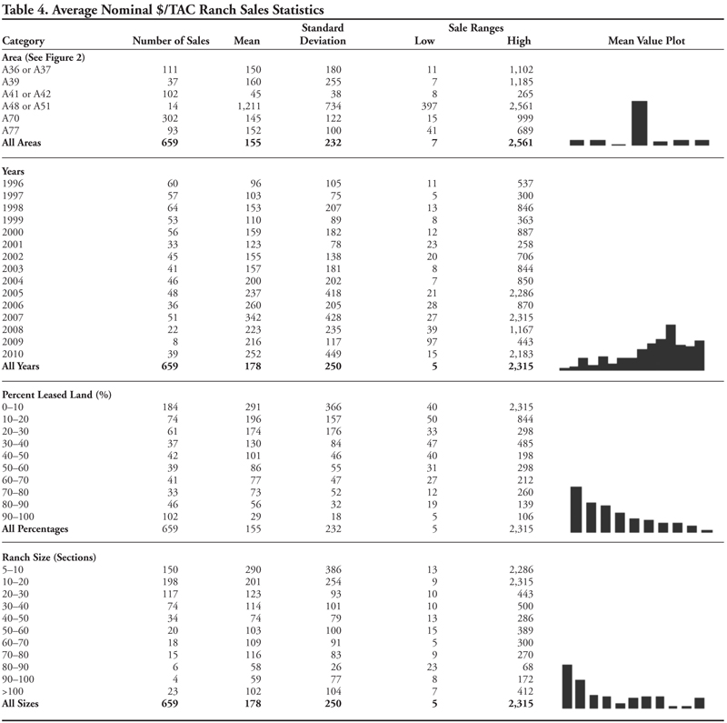
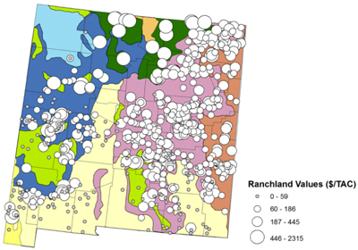
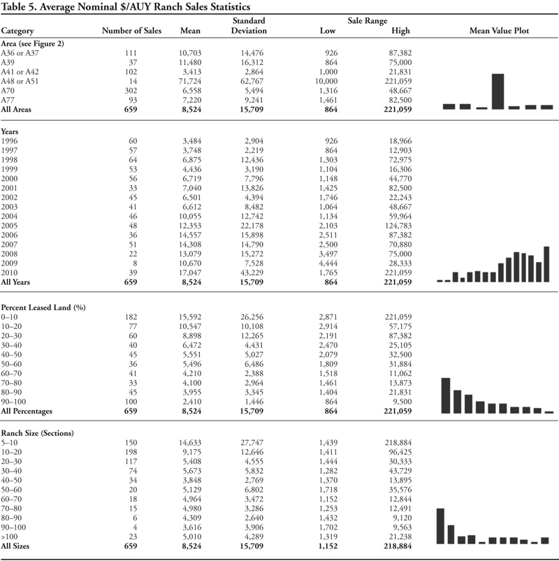
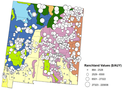
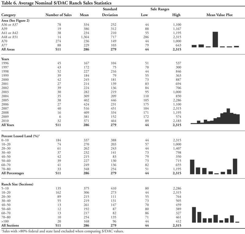
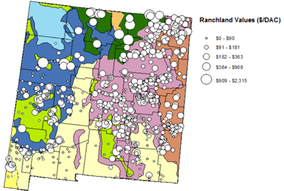
The market value of ranches in the Southern Rocky Mountains (referred to as areas A48 and A51, High Intermountain Valleys in Figure 2) averaged $1,211/TAC, which was nearly 10 times the average for other areas (Table 4). As noted earlier, five additional sales in this area with even higher prices were considered outliers and excluded from the analysis and data. With only 14 ranch sales included for the northern region, the sample size is limited, and thus statistical reliability for the northern region is limited. These sales are in a region that is considered to have exceptional scenic views and the unique cultural amenities of northern New Mexico.
The Pecos Canadian Plains Valley (A70), located in the east-central part of the state (Figure 2) and considered to be one of the most productive rangeland areas for grazing (Stucky and Henderson, 1969), had the highest number of sales at 302. Ranch sale prices in the major livestock-producing areas of the Pecos Canadian Plains Valley and the Southern High Plains (A77) tended to be highest in the northeast corner of the production area, where rangeland productivity is highest (Stucky and Henderson, 1969) and the percentage of deeded land on the ranch is relatively high (Figure 3). Ranches in the southern part of the state generally depended on state, BLM, and USFS lands for over 50% of their grazing capacity (Figure 4).
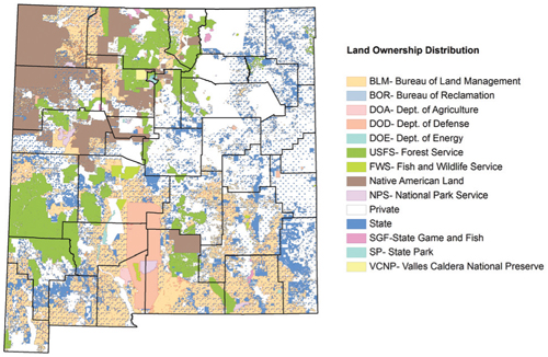
Figure 3. Land ownership in New Mexico (University of New Mexico, 2011).
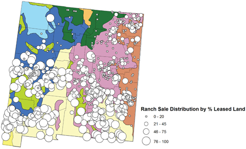
Figure 4. Spatial distribution of ranch sales by percentage of land from state, BLM, and USFS.
The lowest-valued rangeland was in the southern part of the state (A41 and A42), averaging $45/TAC ($3,413/AUY). Ranches in this area are primarily desert ranches that depend heavily on forage leased from the BLM and state trust land (Figure 3). As an average, the sample ranches in the southern desert area depended on BLM lands for 50% of their grazing capacity, state lands for 28%, and deeded lands for 22%.
Average ranch sale prices were relatively constant at about $100 to $160/TAC until about 2004 when they began to rise sharply (Tables 4 through 6); this is consistent with pasture values reported by USDA-NASS (Figure 1). Average $/TAC prices increased from $96/TAC in 1996 to the highest price of $342/TAC in 2007 before declining to $216/TAC in 2009. The number of sales in 2009 was limited, with only eight sales included that year. Further, the number of sales and the characteristics of sales were not the same in each year of study, and statistical differences across time are more appropriately analyzed as follows using the hedonic regression model.
Annual Ranch Income
Agricultural income (or, more accurately, non-wildlife income [NETAGTAC]) averaged $1.81/TAC ± $2.08 standard deviation (SD) (Table 3). As would be expected, income from livestock production closely followed the carrying capacity of rangelands across the state, and was highest in the northeast corner of the state where rangelands are the most productive (Stucky and Henderson, 1969) (Figure 5). Ranches reporting crop income tended to be in eastern New Mexico or the central northern mountains.
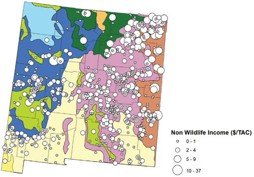
Figure 5. Spatial distribution of non-wildlife income ($/TAC).
Wildlife income averaged $0.44/TAC ± $1.37 (Table 3), with 36% of the sample ranches reporting wildlife income earning potential. Ranches with the largest per acre income from wildlife hunting permits had elk permits and were located in mountainous areas (Figure 6).
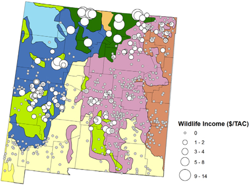
Figure 6. Spatial distribution of wildlife income ($/TAC).
Hedonic Model Parameter Estimates
Parameter estimates for the truncated hedonic model are shown in Table 7. SAS software diagnostics did not indicate a serious problem with multicollinearity, but an unequal variance (heteroscedasticity) was problematic based on the White test (P < 0.001). Thus, White’s heteroscedasticity consistent estimator of the variance-covariance matrix was used for hypothesis testing. Residual plots did not show an undesired pattern when plotted against key factors, including time of sale, amount of leased public land, ranch size, elevation, or MLRA ranching area.
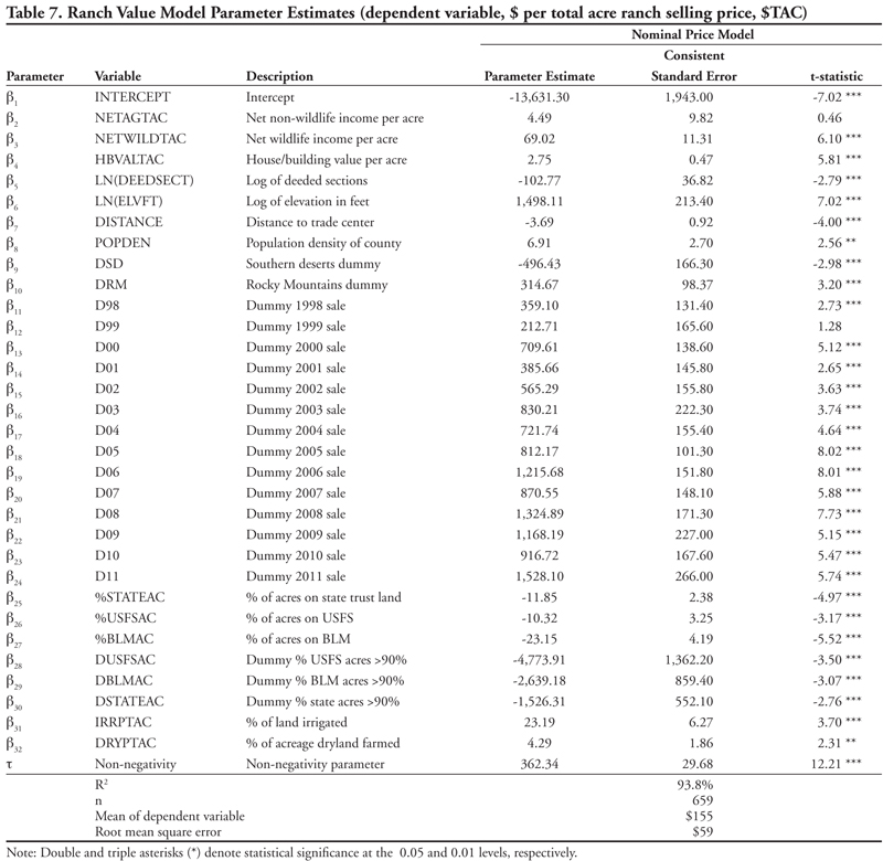
Several of the trend and location dummy variables were not significant (P < 0.10) and were thus excluded. Initial regressions indicated 1996 and 1997 sale prices were not statistically different, so D9 was excluded from the final model. The time dummy variables shift the intercept relative to a 1996 to 1997 base period.
The non-negativity parameter (τ) was highly significant in the truncated model (P < 0.001). The R2 of the model increased from about 84% for the non-truncated model (not shown) to about 94% with the truncation (Table 7). The root mean square error (RMSE) decreased substantially with the truncated model (from $95/acre to $59/acre). Most importantly, of the total 659 ranch sales included in the analysis, the non-truncated model inappropriately predicted negative values for 57 of the ranch sales.
Statistically significant location dummy variables in the model were the southern desert region (DSD or areas A41 and A42, Figure 2) and the northern mountains (DRM, A48 and A51) (Table 7). As might be expected, southern desert ranches were found to be lower in price relative to other areas, with a parameter estimate for ![]() 9 of −$496, whereas northern mountain ranches were higher in sale price relative to other areas (
9 of −$496, whereas northern mountain ranches were higher in sale price relative to other areas (![]() 10 = +$315). The estimated beta coefficient cannot be interpreted directly as a marginal difference, however. As noted in Appendix A and detailed by Xu et al. (1994), marginal changes in the truncated model will be ranch-specific, depending on site-specific estimates of g(∙) (Equation 1) and the scaling factor. Marginal values are estimated by multiplying the model parameter estimate by the scaling factor estimated for a particular ranch (Rimbey et al., 2007; Equation 3). The scaling factor ranges from zero (0) to one (1), and marginal changes will be larger for relatively high-value ranches where the scaling factor is near one. Over 80% of the sample ranches had a scaling factor estimate of 0.20 or less (Figure 7). The average scaling factor was 0.14. When computed by area, the average scaling factor was near the overall 0.14 average (ranging from 0.13 to 0.16) for all areas except the southern deserts, where it averaged 0.02, and the northern mountains, where it averaged 0.85. Thus, when evaluated at the average for the region, ranches in the southern deserts sold for about $10/TAC less ($−496 × 0.02 = −$9.92) than ranches in other MLRA areas. Ranches in the northern mountains sold for an average of $267/TAC (+$315 × 0.85 = $267.75) more than ranches with similar characteristics but located in one of the other areas without a regional dummy variable included.7
10 = +$315). The estimated beta coefficient cannot be interpreted directly as a marginal difference, however. As noted in Appendix A and detailed by Xu et al. (1994), marginal changes in the truncated model will be ranch-specific, depending on site-specific estimates of g(∙) (Equation 1) and the scaling factor. Marginal values are estimated by multiplying the model parameter estimate by the scaling factor estimated for a particular ranch (Rimbey et al., 2007; Equation 3). The scaling factor ranges from zero (0) to one (1), and marginal changes will be larger for relatively high-value ranches where the scaling factor is near one. Over 80% of the sample ranches had a scaling factor estimate of 0.20 or less (Figure 7). The average scaling factor was 0.14. When computed by area, the average scaling factor was near the overall 0.14 average (ranging from 0.13 to 0.16) for all areas except the southern deserts, where it averaged 0.02, and the northern mountains, where it averaged 0.85. Thus, when evaluated at the average for the region, ranches in the southern deserts sold for about $10/TAC less ($−496 × 0.02 = −$9.92) than ranches in other MLRA areas. Ranches in the northern mountains sold for an average of $267/TAC (+$315 × 0.85 = $267.75) more than ranches with similar characteristics but located in one of the other areas without a regional dummy variable included.7
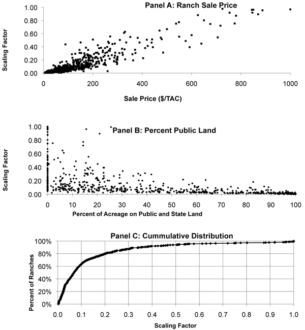
Figure 7. Distribution of estimated scaling factor values.
Similar to the earlier model of Torell et al. (2005), the number of deeded sections and the ranch headquarters elevation (both estimated in natural log form) were statistically important factors explaining ranch value differences. Larger ranches sold for more in total but less on a $/TAC basis, with prices decreasing as the number of deeded sections decreased. Ranches increased in price at a decreasing rate as elevation decreased. Also similar to earlier results, when evaluated at the average scaling factor, increasing the distance to a trade center by 1 mile decreased the value of a ranch by an estimated $0.52/TAC (0.14 × [![]() 7= −$3.69] = −$0.52/TAC). Locating the ranch in a more densely populated county increased per acre value (P < 0.05). Irrigated and dryland farmland included on the property increased the sale price (P < 0.05).
7= −$3.69] = −$0.52/TAC). Locating the ranch in a more densely populated county increased per acre value (P < 0.05). Irrigated and dryland farmland included on the property increased the sale price (P < 0.05).
Torell et al. (2005) found roughness of terrain to be a statistically important factor influencing ranchland values in New Mexico. Roughness was not significant in the updated model and was excluded. The variable PROD (measuring average rangeland carrying capacity) was also not significant and was excluded, whereas it had been significant in earlier models. A new variable included in the updated analysis, distance to a paved road, was not statistically significant and was excluded in the final model.
The conceptually important variable of agricultural income (NETAGTAC), while of the correct positive sign (![]() 2= +$4.49), was not statistically significant in the updated model, but was left in the model given strong theoretical justification. Torell et al. (2005) found agricultural income to be statistically significant (P < 0.01) over the 1990 to 2002 period, with the nominal price coefficient estimated to be +$17. Livestock production value appears to be of less importance over time, as others have also noted (Gentner and Tanaka, 2002; Gosnell and Travis, 2005), and this finding supports that contention. In contrast, farm income has been noted as a major contributor to recent increases in farmland values (AAEA, 2011).
2= +$4.49), was not statistically significant in the updated model, but was left in the model given strong theoretical justification. Torell et al. (2005) found agricultural income to be statistically significant (P < 0.01) over the 1990 to 2002 period, with the nominal price coefficient estimated to be +$17. Livestock production value appears to be of less importance over time, as others have also noted (Gentner and Tanaka, 2002; Gosnell and Travis, 2005), and this finding supports that contention. In contrast, farm income has been noted as a major contributor to recent increases in farmland values (AAEA, 2011).
The wildlife income parameter estimate (![]() 3= +$69) was 15 times larger than the coefficient for non-wildlife income. The 238 ranches with wildlife income had an average scaling factor of 0.26. Evaluated at this average, each dollar of wildlife income added $17.94/acre to ranchland value, suggesting a 5.6% income capitalization rate. At this rate, a $3,000 elk permit would be capitalized into $53,571 in ranch value.
3= +$69) was 15 times larger than the coefficient for non-wildlife income. The 238 ranches with wildlife income had an average scaling factor of 0.26. Evaluated at this average, each dollar of wildlife income added $17.94/acre to ranchland value, suggesting a 5.6% income capitalization rate. At this rate, a $3,000 elk permit would be capitalized into $53,571 in ranch value.
The public and state land discount parameters (β25, β26, β27) for ranches with less than 90% of acreage on leased lands were statistically different from one another (P < 0.0001) using the likelihood ratio-test. Further analysis indicated the acreage discount for USFS and STATE were not different (P = 0.50), while other combinations were different (P < 0.0001). The additional discounts included when leased acreages were greater than 90% (β28, β29, β30) were not statistically different (P = 0.66).
Trends in Ranchland Values
In general, New Mexico ranch value estimates from the hedonic model were found to gradually increase until 2005 when values greatly increased, followed by variable market movements in subsequent years that were not unlike trends in value reported by USDA-NASS (Figure 1). Relative to the previous year, trend variable coefficients decreased in magnitude in 1999, 2001, 2004, 2007, 2009, and 2010 (Table 7). Ranch value estimates are different over time for several reasons beyond the relative value of trend parameter estimates. Different forage lease rates were used to value grazing capacity in alternative years (Table 3), and the estimated scaling factor also varies over time when the estimate of g(X,β) (Equation 1) changes.
Trends in value estimates are most easily seen by considering value estimates for specific ranches of interest. Three different ranches are highlighted using the RANVAL2010 model (Torell, 2011), which can also be used to explore the trend in value for particular ranches of interest. Appendix B provides additional detail about how to use the spreadsheet version of the hedonic model that is available at http://ranval.nmsu.edu. Table 8 gives the RANVAL2010 model inputs used in the valuation for a deeded land ranch in northeast New Mexico (Colfax County), a BLM ranch in southwest New Mexico (Hidalgo County), and a USFS permit ranch in central New Mexico (Lincoln County).
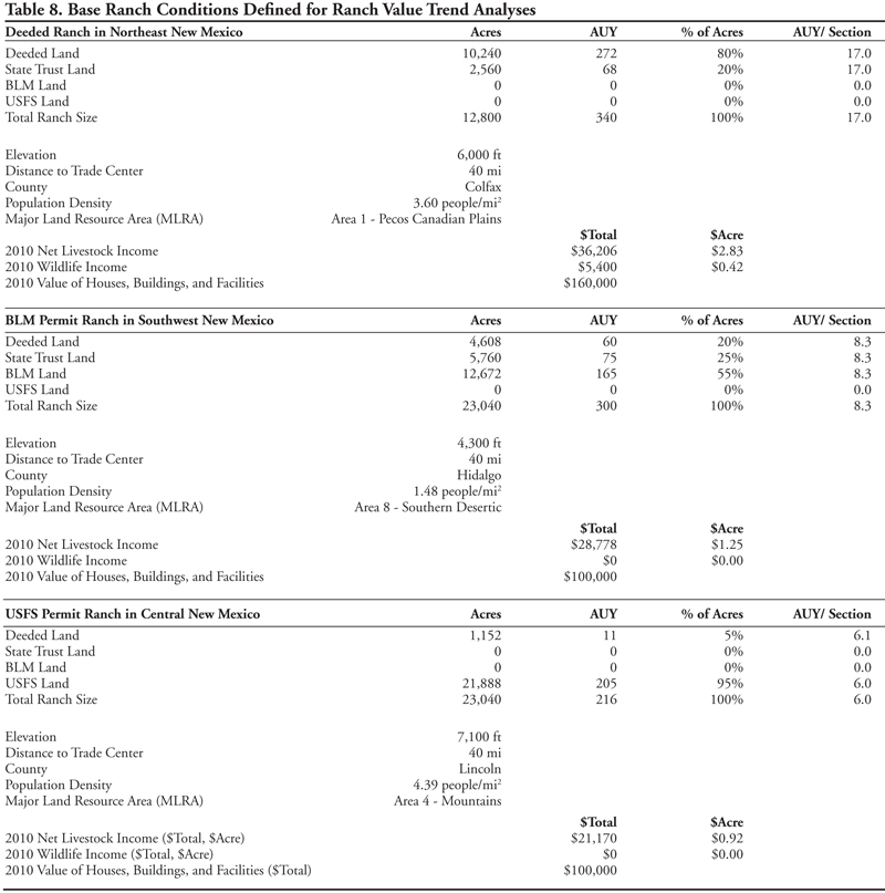
Input parameters are different by area and reflect regional differences in ranch characteristics. We observed wide differences in ranch characteristics, including size of ranch and level of permit land dependency, both within and between geographic regions.
Deeded Land Ranch in Colfax County
The first ranch valuation considers a 20-section ranch in Colfax County whose ranch headquarters is at 6,000 feet elevation (Table 8). The land base is defined to be 80% deeded and 20% state trust land, which would be common in the northeast area (Figure 3). Average carrying capacity of the ranch is defined to be 17 AUY/section, and the ranch has $5,400 ($0.42/acre) in net annual wildlife income from 4 landowner antelope permits. Net income from livestock production is estimated to be $36,206 ($2.83/acre, $106.49/AUY). House, buildings, and facilities on the ranch are estimated to contribute $160,000 ($12.50/acre) to the value of the ranch (in 2010 dollars).
Nominal ranch value estimates increased from $100/TAC ($3,600/AUY) in 1996/1997 to $310/TAC ($11,671/AUY) by July 2010 (Figure 8). Over the study period, nominal prices increased at an annualized rate of 11.1% and real prices increased by 8.9%. Value estimates increased sharply in 2005, diminished during 2006, increased again during 2007, had a downward slide again during 2008 to 2009, and rebounded during 2010. Model estimates follow the same general trend reported by USDA-NASS (Figure 1) and with the same recent market rebound reported by Fay (2011) for other Western ranching areas.
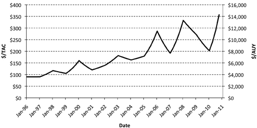
Figure 8. Trend in market value for a deeded land ranch in northeast New Mexico with the characteristics defined in Table 8.
Marginal Value Changes
The nonlinear truncated model definition means that estimated marginal changes in ranch value will be ranch-specific depending on estimates of g(·) (Equation 1) and the model scaling factor. To estimate marginal changes in ranchland value, different scenarios were considered in the RANVAL2010 model by changing selected characteristics of the ranch. Table 9 shows the estimated July 2010 value change for the 20-section Colfax County ranch. With the baseline conditions defined for the ranch, the July 2010 estimate of baseline value was $3,968,073. The scaling factor was estimated to be 0.3978.
Moving the ranch from Colfax County (with a population density of 3.6 people/mi2) to Harding County (population density of 0.34 people/mi2) reduced the estimated ranch value by $112,507 ($8.79/acre). A dollar’s worth of appraised house and building value added $1.10 to ranchland value. Increasing wildlife income by $1,500 added an estimated $37,413 to ranch value, whereas adding an equivalent amount of non-wildlife income added $2,421 to ranch value (Table 9).

As noted with the earlier truncated model estimated by Torell et al. (2005), and with additional discussion in Rimbey et al. (2007), as the initial amount of leased land on a ranch decreases, the contributory value of federal and state land grazing permits is estimated to decrease. The added grazing capacity on public and state lands increases land value, but the percentage of land on leased lands also increases, and this increased leased land dependency has a price discount in the marketplace.
Rimbey et al. (2007, Figure 4) found that adding a state land grazing permit to a mostly deeded land New Mexico ranch (>80% deeded land) would decrease ranchland value. Grazing permit values were estimated to be negative for BLM and USFS permits until about 50% of the ranch acreage was on public land. Similarly, Sunderman and Spahr (1994) concluded that grazing permits diminish ranch value when only a small amount of public land is included on the ranch. Similar results were obtained in our updated model. Adding a section of deeded land to the ranch increased the July 2010 ranch value estimate by $209,428 ($327/acre) (Figure 9). This is in contrast to the −$78/acre value change estimate when state trust land was added to the model (triangle shape in Figure 9). When the ranch started with 33% of acreage on state trust land (instead of the assumed 20% used in the base analysis) the permit value estimate became positive. Permit value increased over the relevant range of leased land dependency (Figure 9). Adding state land acreage to a 20-section Colfax County ranch with 50% of its acreage on state land increased the land value estimate by $61/acre ($2,309/AUY); adding the acreage to a ranch with 70% of the land base on state trust land added $103/acre ($3,880/AUY) (Figure 9).
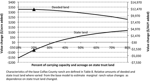
Figure 9. Marginal change in July 2010 ranch value from adding more land to the defined northeast New Mexico ranch.
BLM Permit Ranch in Hidalgo County
The second ranch valuation considers a 36-section (300 AUY) BLM permit ranch (Table 8) located in the southern Desertic Basins MLRA (Figure 2) in Hidalgo County. The land base is defined to be 20% deeded land, 25% state trust land, and 55% BLM land. A relatively high mix of state and BLM land is common in the southern desert area (Figure 3). Average carrying capacity of the ranch is defined to be 8.34 AUY/section. No wildlife income is included. Net income from livestock production is estimated to be $28,778 ($1.25/acre, $96/AUY). The 2010 house, buildings, and facilities investment on the ranch is considered to be $100,000 ($4.34/acre).
We estimate a relatively slow rate of increase in ranchland value for the desert ranch, given the relatively high amount of leased public and state land. Nominal ranch value estimates increased from about $37/TAC ($2,827/AUY) in 1996 to $55/TAC ($4,246/AUY) in July 2010 (Figure 10). Over the study period, estimated nominal prices increased at an annualized rate of 3.6%, or 1.6% after adjusting for inflation.
Marginal Value Changes
With the baseline conditions defined for the desert BLM ranch (Table 8), the July 2010 estimate of ranch value was $1,274,888 (Table 10). Given the relatively low ranch value estimate and the resulting small scaling factor (0.0223), marginal changes from altering ranch characteristics are estimated to be minimal. A 10-mile increase in the distance to town was estimated to decrease total ranch value by $1,872/added mile (Table 10), whereas the change for the 20-section Colfax County ranch was about 10 times more. Moving the ranch from sparsely populated Hidalgo County to the higher density of Doña Ana County increased the value estimate by over $200,000.

Adding another section of rangeland with a carrying capacity of 8.34 AUY/section increased the July 2010 value estimate of the desert ranch by $79/acre if it was deeded land that was added and by $64/acre and $39/acre if it was state or BLM land added, respectively (Table 10). Estimated on an AUY basis, the added acreage and grazing capacity contributed $6,091/AUY if on deeded land, $4,886/AUY if on state trust land, and $2,958/AUY if on BLM land (triangle shape in Figure 11). But the hedonic model results suggest very little of the ranchland value actually came from livestock production. Adding a dollar of annual ranch income added only $0.09/acre to ranchland value (Table 10). Less than 1% of the total value of the ranch is estimated to come from livestock production value. As described by Torell et al. (2007), it is the additional acreage that contributes most to ranchland value. Sunderman and Spahr (1994) found Wyoming ranches to exhibit a similar valuation; additional acreage contributed to the value of Wyoming ranches even with little, if any, increase in ranch grazing capacity. Similar results were found for Great Basin ranches (Rimbey et al., 2007). The importance of livestock production in determining ranchland values is diminishing.
Similar to state land permit value estimates for the Colfax County ranch (Figure 10), permit value estimates for the desert BLM ranch declined when the permit was added to a ranch with increasing amounts of deeded land in the initial land base (Figure 11). The July 2010 value of the state trust land permit was estimated to be relatively constant at about $63/acre ($4,884/AUY) if the ranch started with over 40% of the acreage on leased BLM and state trust land. Deeded land and state trust land contributed nearly the same amount when the 36-section ranch had 90% of acreage on leased lands (Figure 11). A positive BLM permit value was realized when the base ranch had about 40% of the acreage on leased lands. The BLM permit value increased to about $40/acre ($3,000/AUY) when added to a ranch with 90% of its acreage on state and BLM land (Figure 11).
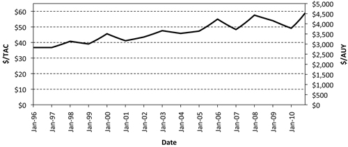
Figure 10. Trend in market value for BLM ranch in southwest New Mexico with the characteristics defined in Table 8.
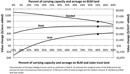
Figure 11. Marginal change in July 2010 ranch value for a 32-section Hidalgo County ranch with different relative amounts of deeded, state, and BLM land included.
USFS Permit Ranch in Lincoln County
The final hedonic model estimation is for a USFS permit ranch in Lincoln County. The sample size for USFS ranches in the database was limited, with only 44 sales. Seventeen of the 44 sales had over 90% of their acreage on USFS lands. Consistent with the characteristics of the sales in the database, a 36-section USFS ranch with a carrying capacity of 6 AUY/section (216 AUY) is considered (Table 8). Ninety-five percent of the grazing capacity is considered to be on USFS land. As with the Hidalgo BLM ranch considered in the second valuation, the high percentage of USFS land means a relatively low-value ranch with marginal impacts from altering ranch characteristics. Marginal changes in value were not evaluated, and with the nearly constant estimate of value, detail about the value change over time is also not shown.
The defined USFS ranch had an estimated total value of $479,500 ($20.81/TAC, $2,220/AUY) in 1996, with an increase in value to about $600,000 ($26/TAC, $2,750/AUY) by 2010. On a nominal price basis, the annualized rate of appreciation was 1.85%, nearly equal to the rate of inflation over the period.
Trends in Permit Value
We estimated trends in grazing permit values for the defined Hidalgo County BLM ranch and the Lincoln County USFS ranch by adding one more section (640 acres) of different types of land to the defined models. The contributory values of deeded, state trust, and BLM land were estimated from the Hidalgo County model, and USFS permit value trends were estimated from the Lincoln County model (Table 8). As shown in Figure 12, for the Hidalgo County model, an additional acre of deeded land contributed about an extra $48/acre ($3,670/AUY) of value in 1996, and this value increased to about $79/acre ($6,100/AUY) by July 2010. The contributory value of the state land grazing permit on the Hidalgo County ranch increased from $40/acre ($3,120/AUY) in 1996 to $63/acre ($4,884/AUY) in 2010. The value of the BLM permit rose more slowly in value, from about $30/acre ($2,329/AUY) in 1996 to about $40/acre ($3,000/AUY) in 2010. Adjusting for inflation (detail not shown), the estimated value of the BLM permit stayed relatively constant at about $40/acre in 2010 dollars.
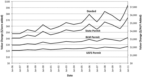
Figure 12. Trends in grazing permit values, 1996 to 2010.
For the Lincoln County ranch model, the marginal value contribution from the USFS permit was relatively constant at about $20/acre ($1,500/AUY). Values increased at 1.85% per year, slightly less than the rate of inflation over the period. Earlier New Mexico hedonic models estimate the same nearly constant real-price permit value contributions for BLM and USFS lands going back to the early 1980s (Rimbey et al., 2007).
Discussion
This research updated earlier New Mexico hedonic ranch value models. Many of the factors previously found to influence ranchland values continue to be important, such as the amount of state and public land included on the ranch, ranch size and location, and hunting opportunities. Livestock earning potential of the ranch was found to be of declining importance in determining ranchland values and was not found to be statistically significant in the updated hedonic model estimated here, though it was significant in earlier New Mexico models (Torell et al., 2005). The declining importance of livestock income in determining pasture and rangeland values is consistent with the findings of Doye and Brorsen (2011), who note that pasture land values throughout the nation are now influenced by amenity and development factors. Many urban dwellers have an affinity for country living and are willing to pay a premium price for grazing lands. Current ranch buyers seek income earning potential, recreational opportunities, and the desired open space and agrarian lifestyle that owning a Western ranch provides. The lifestyle influence is not new, however. Martin and Jefferies (1966) noted its influence on the price of Arizona ranches back in the early 1960s.
Market influences beyond just livestock production are obvious when the average price of New Mexico ranches is about $8,500/AUY (Table 3) as compared to annual ranch income levels of about $100/AUY, an implied 1.2% capitalization rate. Nationwide rent-to-value ratios for pasture lands have also fallen to about 1% (Doye and Brorsen, 2011). Yet, contrary to the findings of diminished income earning influences for New Mexico ranches, cropland values have seen recent increases, and those increases have been driven by strong agricultural commodity demand and income, low interest rates, and a lack of alternative high-yield investments (AAEA, 2011; Messick, 2011).
With livestock production returns in the 1 to 3% range on a real-price basis (Torell et al., 2001), land appreciation has been an important part of the return traditionally realized from ranchland investment. The nonlinear truncated model results suggest lower rates of land appreciation for relatively low-value public land ranches as compared to deeded land ranches that are in scenic mountainous locations with substantial hunting and recreational opportunities. This is consistent with the observations of Wheeler (2011), who notes there is a segment of the ranch real estate market that is production-based, and these relatively low-value ranches have not increased or decreased much in value. He also notes substantial and continued increases in high-valued recreational ranches.
The definition of the truncated model is limited because it does not allow livestock production income to be of greater importance for relatively low-value ranches. It might be expected that the purchase of a permit ranch is primarily for livestock production. To the contrary, the defined functional form of the hedonic model suggests all marginal price influences will be more substantial as characteristics change to increase ranchland value. Yet including the truncation in the hedonic model resulted in a 10% increase in the model R2, and residual plots did not indicate discernible residual patterns for different kinds of ranches.

Acknowledgements
This research was supported by the U.S. Forest Service Rocky Mountain Research Station under Grant No. 01-JV-11221617-273FS and by the New Mexico State University Agricultural Experiment Station. Farm Credit Services was especially generous in providing ranch sales data for this study. In particular, we are grateful to Greg Carrasco, Richard Armijo, Jim Welles, and Colin McVeigh for their assistance.
Literature Cited
AAEA. 2011. December 13, 2011: AAEA Extension Section & C-FARE- Regional perspectives on economic forces shaping land asset values [Webinar]. Retrieved December 17, 2011, from http://www.farmmanagement.org/aginuncertaintimesenglish/2011/12/13/2214/
Anselin, L., and A.K. Bera. 1998. Spatial dependence in linear regression models with an introduction to spatial econometrics. In A. Ullah and D.E.A. Giles (Eds.), Handbook of applied economic statistics, (vol. 155, pp. 237–289). New York, NY: Marcel Dekker.
Anselin, L., and N. Lozano-Gracia. 2008. Errors in variables and spatial effects in hedonic house price models of ambient air quality. Empirical Economics, 34, 5–34.
Appraisal Institute and ASFMRA. 2000. The appraisal of rural property, 2nd ed. Chicago, IL.
Baird, F.P. 2010. Montana agricultural land prices: An evaluation of recreational amenities and production characteristics [Thesis]. Bozeman, MT: Montana State University.
Bartlett, E.T., L.A. Torell, N.R. Rimbey, L.W. Van Tassell, and D.W. McCollum. 2002. Valuing grazing use on public land. Journal of Range Management, 55, 426–438.
Bastian, C.T., D.M. McLeod, M.J. Germino, W.A. Reiners, and B.J. Blasko. 2002a. Environmental amenities and agricultural land values: A hedonic model using geographic information systems data. Ecological Economics, 40, 337–349.
Bastian, C.T., W.A. Reiners, B.J. Blasko, D.M. McLeod, and M.J. Germino. 2002b. Exploring the potential for using GIS to measure environmental and visual amenities when valuing agricultural lands. Journal of the American Society of Farm Managers and Rural Appraisers, 65, 43–52.
Bergstrom, J.C., and R.C. Ready. 2009. What have we learned from over 20 years of farmland amenity valuation research in North America? [Online]. Review of Agricultural Economics, 31, 21–49.
Burt, O.R. 1986. Econometric modeling of the capitalization formula for farmland prices. American Journal of Agricultural Economics, 68, 10.
Collins, A.R. 1983. A ranch land price model for Wyoming [Report SM44R]. Laramie, WY: University of Wyoming Agricultural Experiment Station.
Donovan, G.H., D.T. Butry, and P.A. Champ. 2007. Wildfire risk and housing prices: A case study from Colorado Springs. Land Economics, 83, 217–233.
Doye, D., and B.W. Brorsen. 2011. Pasture land values: A “Green Acres” effect? [Online]. Retrieved October 13, 2011, from http://www.choicesmagazine.org/choices-magazine/theme-articles/farmland-values/pasture-land-values-a-green-acres-effect
Duffy, M. 2011. The current situation on farmland values and ownership [Online]. Retrieved October 13, 2011, from http://www.choicesmagazine.org/choices-magazine/theme-articles/farmland-values/the-current-situation-on-farmland-values-and-ownership
Egan, L.M., and M.J. Watts. 1998. Some costs of incomplete property rights with regard to federal grazing permits. Land Economics, 74, 171–185.
Fay, G.W. 2011, April 29. State of the ranch market and spring 2011 newsletter [Online]. Retrieved July 9, 2011, from http://fayranches.com/blog/2011/04/29/state-ranch-market-and-spring-2011-newsletter
Gardner, B.D. 1997. Some implications of federal grazing, timber, irrigation, and recreation subsidies. Choices, 3, 9–14.
Gentner, B.J., and J.A. Tanaka. 2002. Classifying federal public land grazing permittees. Journal of Range Management, 55, 2–11.
Google. 2011. Google Maps [Online]. Retrieved August 24, 2011, from http://maps.google.com/
Gosnell, H., and W.R. Travis. 2005. Ranchland ownership dynamics in the Rocky Mountain West. Rangeland Ecology and Management, 58, 191–198.
Gosnell, H., J. Haggerty, and W. Travis. 2006. Ranchland ownership change in the greater Yellowstone ecosystem, 1990–2001: Implications for conservation. Society & Natural Resources, 19, 743–758.
Gosnell, H., J.H. Haggerty, and P.A. Byorth. 2007. Ranch ownership change and new approaches to water resource management in southwestern Montana: Implications for fisheries. Journal of the American Water Resources Association, 43, 990–1003.
Grazing Leases and Permits, 43 U.S.C. § 1752. 2010.
Henderson, P. 2000, February. The lure of land: Investors are buying their own piece of heaven [Online]. Top Producer. Retrieved June 8, 2000.
Kelejian, H.H., and D.P. Robinson. 1992. Spatial autocorrelation: A new computationally simple test with an application to per capita county police expenditures. Regional Science and Urban Economics, 22, 317–331.
Kilpatrick, J.A. 2004. Real estate issues in class certification [Online]. Retrieved June 17, 2011, from http://www.greenfieldadvisors.com/our-work/journal-articles/109-real-estate-issues-in-class-certification
Madsen, A.G., C.K. Gee, and J.B. Keffeler. 1982. Market vs. productive value of Colorado ranches. Journal of American Society of Farm Managers and Rural Appraisers, 46, 19–23.
Martin, W.E. 1966. Relating ranch prices and grazing permit values to ranch productivity. Journal of Range Management, 19, 248–252.
Martin, W.E., and G.L. Jefferies. 1966. Relating ranch prices and grazing permit values to ranch productivity. Journal of Farm Economics, 48, 233–242.
Melichar, E. 1979. Capital gains versus current income in the farming sector. American Journal of Agricultural Economics, 61, 1,085–1,092.
Messick, M. 2011, December 22. As farmland prices soar, it’s not just farmers buying [Online]. Retrieved January 19, 2012, from http://stateimpact.npr.org/idaho/as-farmland-prices-soar-it%E2%80%99s-not-just-farmers-buying/
Mueller, J.M., and J.B. Loomis. 2008. Spatial dependence in hedonic property models: Do different corrections for spatial dependence result in economically significant differences in estimated implicit prices? Journal of Agricultural and Resource Economic, 33, 212–231.
New Mexico Department of Game and Fish. 2004. Land owner list for elk private lands use system (E-PLUS) and antelope private lands use system(A-PLUS) [Online]. Retrieved August 31, 2011, from http://www.wildlife.state.nm.us/recreation/hunting/index.htm
Patton, M., and S. McErlean. 2003. Spatial effects within the agricultural land market in Northern Ireland. Journal of Agricultural Economics, 54, 35–54.
Poniewozik, J. 2005. America’s house party [Online]. Time Magazine. Retrieved July 9, 2011, from http://www.time.com/time/magazine/article/0,9171,1069097,00.html
Pope, C.A. 1985. Agricultural productive and consumptive use components of rural land values in Texas. American Journal of Agricultural Economics, 67, 81–86.
Rimbey, N.R., L.A. Torell, and J.A. Tanaka. 2007. Why grazing permits have economic value. Journal of Agricultural and Resource Economics, 32, 20–40.
Sands, L. 1998. Pearls beyond price: The West’s pristine ranches set new highs [Online]. Top Producer Magazine. Retrieved June 8, 2000.
Smith, A.H., and W.E. Martin. 1972. Socioeconomic behavior of cattle ranchers with implications for rural community development in the West. American Journal of Agricultural Economics, 54, 217–225.
Stucky, H.R., and D.C. Henderson. 1969. Grazing capacities and selected factors affecting public land use [Research Report 158]. Las Cruces, NM: New Mexico State University Agricultural Experiment Station.
Sunderman, M.A., and R.W. Spahr. 1994. Valuation of government grazing leases. Journal of Real Estate Research, 9, 179–196.
Sunderman, M.A., R.W. Spahr, J.W. Birch, and R.M. Oster. 2000. Impact of ranch and market factors on an index of agricultural holding period returns. Journal of Real Estate Research, 19, 209.
Taylor, L.O. 2003. The hedonic method. In P.A. Champ, K.J. Boyle, and T.C. Brown (Eds.), A primer on nonmarket valuation (pp. 331–394). Dordrecht, The Netherlands: Kluwer Academic Publishers.
Torell, L.A. 2011. RANVAL 2010: A hedonic model for predicting the market value of New Mexico ranches, 1996–2010 [Online]. Retrieved August 1, 2011, from http://ranval.nmsu.edu
Torell, L.A., and S.A. Bailey. 2000. Is the profit motive an important determinant of grazing land use and rancher motive? [Online]. Selected paper presented at the Western Agricultural Economics Association 2000 Annual Meeting, June 29- July 1, 2000, Vancouver, B.C. Retrieved June 28, 2011, from http://ageconsearch.umn.edu/handle/36451
Torell, L.A., and J.P. Doll. 1990. The market value of New Mexico ranches, 1980-88 [Bulletin 748]. Las Cruces, NM: New Mexico State University Agricultural Experiment Station.
Torell, L.A., and J.P. Doll. 1991. Public land policy and the value of grazing permits. Western Journal of Agricultural Economics, 16, 174–184.
Torell, L.A., and J.M. Fowler. 1986. A model for predicting trends of New Mexico grazing land values [Bulletin 723]. Las Cruces, NM: New Mexico State University Agricultural Experiment Station.
Torell, L.A., I.T. Pearson, and S.A. Bailey. 2000. New Mexico ranch values: RANVAL 2000 [Online]. Retrieved September 7, 2010, from http://ranval.nmsu.edu/RANVAL2000.xls
Torell, L.A., N. Rimbey, and O.A. Ramirez. 2003. RANVAL 2003: A model for estimating New Mexico ranchland values [Online]. Retrieved June 1, 2011, from http://ranval.nmsu.edu/Ranval2003v6.xls
Torell, L.A., N.R. Rimbey, O.A. Ramirez, and D.W. McCollum. 2005. Income earning potential versus consumptive amenities in determining ranchland values. Journal of Agricultural and Resource Economics, 30, 537–560.
Torell, L.A., N.R. Rimbey, J.A. Tanaka, and S.A. Bailey. 2001. The lack of a profit motive for ranching: Implications for policy analysis [Online]. In L.A. Torell, E.T. Bartlett, and R. Larrañaga (Eds.), Proceedings of the Annual Meeting of the Society for Range Management: 17-23 February 2001, Kailua-Kona, HI, USA (pp. 47–58). Retrieved November 26, 2009, from http://ageconsearch.umn.edu/handle/16629
University of New Mexico. 2011. New Mexico resource geographic information system (RGIS), land ownership map data [Online]. Retrieved August 31, 2011, from http://rgis.unm.edu/
USDA-NASS. 2012. Agricultural prices monthly [Online]. Retrieved February 1, 2012, from http://usda.mannlib.cornell.edu/MannUsda/viewDocumentInfo.do?documentID=1002
USDA-NASS. Various issues. Agricultural land values and cash rents annual summary [Online]. Retrieved July 8, 2011, from http://usda.mannlib.cornell.edu/MannUsda/%20viewDocumentInfo.do?documentID=1446
USDA-NRCS. 2006. Land resource regions and major land resource areas of the United States, the Caribbean, and the Pacific basin [USDA Handbook 296, Online]. Retrieved August 24, 2011, from http://soils.usda.gov/survey/geography/mlra/
Wasson, J., D.M. McLeod, C.T. Bastian, and B.S. Rashford. 2010. The effects of scenic and environmental amenities on agricultural land values [Online]. Organized symposium paper presented at Quantifying the Determinants of Land Values: The Impacts of Irrigation, Recreational Amenities, and Off-Farm Income, Agricultural & Applied Economics Association’s 2010 AAEA, CAES & WAEA Joint Annual Meeting; Denver, Colorado. Retrieved June 25, 2012, from http://purl.umn.edu/61597
Wheeler, N.C. 2011. General market conditions and sales [Online]. Retrieved July 9, 2011, from http://www.ncwheeler.com/Pages/Market.aspx
Winter, J.R., and J.K. Whittaker. 1981. The relationship between private ranchland prices and public-land grazing permits. Land Economics, 57, 414–421.
Workman, J.P., and K.H. King. 1982. Utah cattle ranch prices. Utah Science, 43, 78–81.
Xu, F., R.C. Mittelhammer, and L.A. Torell. 1994. Modeling nonnegativity via truncated logistic and normal distributions: An application to ranch land price analysis. Journal of Agricultural and Resource Economics, 19, 102–114.
Appendix A: Estimation Issues for Hedonic Ranch Value Models
This appendix describes key estimation issues that have arisen and been recognized as various New Mexico hedonic ranch value models have been developed, starting in 1986 (Table 1). Insight is also provided about how future models might be improved with a more intensive data collection effort and use of GIS data and layers, similar to the modeling efforts of Bastian et al. (2002a).
Defining the Dependent Variable
An important decision is how to define the dependent variable in a hedonic ranch valuation model. Ultimately, the desire is to estimate the total value of a ranch, and some have defined total sale price to be the dependent variable (see for example Martin and Jefferies [1966], Sunderman and Spahr [1994], Torell and Fowler [1986], and Baird [2010]). This is problematic, however, because some estimated model coefficients will be too big for small ranches and too small for large ranches, but accurate near the average size. Many previous hedonic ranch models have standardized the dependent variable to $/deeded acre (see for example Pope [1985] and Bastian et al. [2002a]). This is appropriate for areas with primarily deeded lands. However, in public land ranching areas, the price per deeded acre is misleading because a ranch with few deeded acres and large public and state land permits attached will have high prices per deeded acre even though the majority of value comes from grazing permits. In early New Mexico models (Table 1) and in other studies (Workman and King, 1982), the dependent variable was defined on a $/livestock unit basis (e.g., $/AUM, $/AUY, $/brood cow). This is appropriate when most of the economic value comes from livestock production, but Western ranches now have value far in excess of expected discounted income from livestock production. Torell et al. (2005) and Rimbey et al. (2007) defined the dependent variable in the hedonic model to be $/total acre ($/TAC), dividing the total sale price by the deeded, state, and public land acreages included with the sale. This standardizes the dependent variable and recognizes that value comes from various types of land. An obvious criticism is that clear title to public and state lands is not acquired at ranch purchase. Further, while the number of AUMs and land acreage provided from state and public lands is available in land agency databases, many times the land acreage is not reported on ranch appraisal sheets, requiring additional data collection effort.
Non-Negativity Restriction
In most cases land values will not be negative8, and thus the distribution of the error term in the hedonic model should not allow for a negative dependent value. The model should be truncated with zero as the lower limit land value. This has proven to be especially important when hedonic ranch models are estimated on a $/TAC basis because ranches with primarily public lands have $/TAC values that are relatively close to zero. Earlier research papers described how to estimate the truncated model and described the complications that arise in estimating marginal impacts of the various explanatory variables (Xu et al., 1994; Torell et al., 2005; Rimbey et al., 2007). This detail is not repeated here except to note that the truncated nonlinear model means the marginal impacts from changing ranch characteristics will be ranch-specific. The scaling factor (D-function value) of the model ranges from zero (0) to one (1) and will be near 1 for relatively high-value ranches and near 0 for low-value ranches. As an example, this means that adding additional houses and buildings to a high-value deeded land ranch will mean a bigger estimated change in ranch value than adding improvements to a relatively low-value public land ranch. The change in marginal impacts results from the defined functional form of the truncated model, and it may or may not be appropriate.
Spatial Autocorrelation
Correcting for autocorrelation in time series models has a long history. Only recently, and largely relying on spatial geographical information system (GIS) data, have researchers begun to correct for spatial autocorrelation (Anselin and Bera, 1998). Spatial error dependence and spatial lag dependence are two forms of spatial autocorrelation. Spatial error dependence occurs where the dependence pertains to the error terms, whereas spatial lag dependence occurs where the dependence pertains to the dependent variable (Patton and McErlean, 2003). Failure to correct for a spatial lag process (when present) results in biased coefficient estimates, and failure to correct for spatially correlated errors results in inefficient coefficient estimates (Mueller and Loomis, 2008).
Due to a circularity of price setting, the agricultural land market is a case where spatial error dependence may exist. Property owners, prospective buyers, real estate brokers and appraisers, and others may base their estimate of property value partly on observed comparable recent sales in the area. This suggests that the value of a real estate property depends not only on its own characteristics but also on the characteristics and amenities of surrounding properties (Patton and McErlean, 2003; Mueller and Loomis, 2008).
Several recent real estate studies have considered and corrected for spatial autocorrelation with applications to housing markets (Donovan et al., 2007; Anselin and Lozano-Gracia, 2008; Mueller and Loomis, 2008), the farmland market (Patton and McErlean, 2003), and the Western ranch real estate market (Bastian et al., 2002a; Baird, 2010; Wasson et al., 2010). The importance of the correction for spatial correlation in ranch applications is mixed, but it does not generally show large differences in parameter estimates for corrected versus uncorrected models. Bastian et al. (2002a) found no spatial correlation for ranches located within 400 miles of each other, but additional tests using smaller distance bands9 were not possible because of additional problems with heteroscedasticity and because diagnostics for spatial correlation are questionable in the presence of heteroscedasticity. When heteroscedasticity is present, the spatial autocorrelation test proposed by Kelejian and Robinson (1992) (K-R test) can be used to find the relevant spatial distance band. Wasson et al. (2010) used this procedure and Wyoming ranch sales data collected from Farm Credit Services over the 1989 to 1995 period (the same data source or subset of data used by Bastian et al. [2002a]) to conclude that the appropriate spatial distance band was 54 miles. They corrected for both heteroscedasticity and spatially correlated errors in the hedonic model using feasible generalized least squares (FGLS) procedures. They noted that the corrected model improved model efficiency and goodness of fit but did not comment on the magnitude of the differences between corrected and uncorrected model parameter estimates.
When using a distance band of 60 miles or fewer for Montana ranch sales, Baird (2010) found significant spatial lag dependence in hedonic ranchland models estimated in logarithmic functional form. He found, however, that correcting for spatial lag dependence had little consequence on defining which variables would be considered statistically significant in the equations or the magnitudes of statistically significant coefficients. Similarly, Mueller and Loomis (2008) found relatively small differences between ordinary least squares (OLS) price estimates relative to those estimated from spatially corrected models. They concluded that the inefficiency of OLS estimation in the presence of spatially correlated errors may not always be economically significant and that non-spatial hedonic property models can provide useful results.
Improving Future Hedonic Ranch Valuation Models
The steps required to substantially improve hedonic ranch valuation models will mean a more intensive definition of ranch characteristics and a costlier data collection effort. As demonstrated by Bastian et al. (2002a, 2002b), Wasson et al. (2010), and Baird (2010), GIS data have potential in further defining additional ranch characteristics that can be related to sale price differences. Similar to the environmental, wildlife habitat, and scenic view variables considered by these authors in hedonic models, GIS layers could potentially define productivity and brush canopy characteristics of rangeland acres on study ranches. Differences in landscape characteristics between ranches could then potentially be used to evaluate how reducing brush canopy influences ranchland values. Other ecosystem services provided from rangelands could be valued in a similar way. GIS-based procedures and tests are also required to test for and correct for the problems of spatial correlation described previously.
The growing importance of recreational and wildlife opportunities in setting ranchland values suggests an expanded effort in defining those opportunities for each ranch sale. Farm Credit Service appraisers did not record wildlife income for all ranch sales. Many of those sales that excluded this information likely had no marketable hunting opportunities on the ranch, but some did. Excluding wildlife income in some cases potentially biases the parameter estimate for wildlife income. An alternative would be to define the acreage of particular wildlife habitat provided on the ranch (Bastian et al., 2002b).
Other factors that would be expected to influence ranch values include the dollar value of range improvements in addition to the house and building values currently recorded on FCS appraisal sheets. Recording the acreage of permitted lands in all cases would be useful, as would defining the season of allowed use for those grazing permits that are not grazed year-round.
The hedonic model used here estimates ranch sale price on a $/TAC basis. This value is a weighted average price contribution of different land types (deeded, BLM, USFS, state trust land). The value of grazing permits is not directly estimated but must instead be estimated by adding more or fewer permitted acres to the model with multiple estimations or by using a complex formula to compute marginal changes (Xu et al., 1994). Using GIS data to define separately the characteristics (e.g., elevation, vegetation, brush canopy, greenness, wildlife habitat provided) of the deeded land and the permitted land would allow inclusion of additional explanatory variables that separately and directly value the deeded and permitted acreages. While the dependent variable may still be total acre price, the modified equation would provide separate parameter estimates for the contributions made by alternative land types. The separate land type components of the total price estimate might be weighted by the acreages from the different land types.
Appendix B: Using RANVAL 2010
An Excel spreadsheet that calculates the hedonic model described in this research report is available at https://pubs.nmsu.edu/research/economics/RR779/documents/RANVAL2010v5.xls The model estimates the market value of New Mexico ranches (>5 sections in size) over the January 1996 to January 2011 period based on user-provided ranch characteristics. Obviously, the validity of the estimate will depend on the accuracy of the data provided. New Mexico State University does not assume responsibility for the accuracy of the model value estimates.
The spreadsheet model uses Excel macros, and the user must enable macros for it to work properly. Figure 13 shows the input screen for the RANVAL2010 model. Links are provided on the input screen to help the user understand the data requested. Only the yellow cells with a black border should be altered; other cells are calculated.
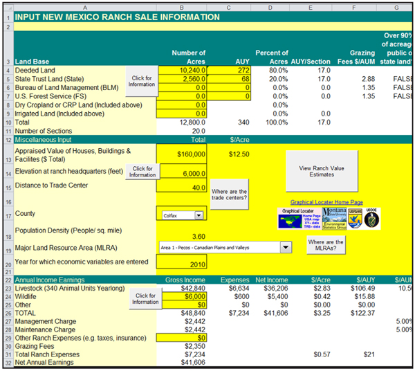
Figure 13. Ranval2010 model input screen.
The first block of data requested is the acreage and carrying capacity rating for deeded, state, BLM, and USFS lands. Irrigated and dryland crop acreages must also be supplied. Additional inputs include the appraised (depreciated) value of houses, buildings, and substantial facilities. The appraised values of fencing and water facilities are not valued directly but rather implied as an average value in the estimation. Distance to the nearest trade center (Table 2) is a required input, as is the elevation of the ranch at the headquarters. Population density is computed by selecting the county location of the ranch headquarters. The NRCS major land resource area where the ranch is located is another required input.
One field (cell B20) asks for the year for which economic variables are entered. If a current estimate (2010-2011) is made, then 2010 (or 2011) should be entered. The model is estimated on a nominal price basis, and economic variables are adjusted for inflation relative to the year specified. Specifically, the amount you enter as a house and building value and for wildlife and other income and expenses will be adjusted for inflation relative to the year specified here. Forage lease rates and grazing fees are also different by year.
Ranch value estimates on both a nominal and real price basis are estimated from the defined model input and can be viewed and printed using either the “View Ranch Value Estimates” button on the input screen or by selecting the “Estimated Values” spreadsheet tab at the bottom of the screen. Quarterly estimates of value are provided from January 1996 through January 2011. The annual rate of appreciation shown at the bottom of the screen is calculated as the annual rate of discount that would cause the estimated January 1996 value to grow to the January 2011 value (a 15-year period).
1An animal unit (AU) is considered to be one mature cow with calf or the equivalent. An animal unit month (AUM) is the amount of forage required for one AU for one month. An animal unit yearlong (AUY) is the forage required for one AU for one year.
2USDA pasture value estimates are for deeded lands and exclude BLM, USFS, and state trust land.
3FCS allows NMSU to use ranch sale information with the understanding that the individual sale records will remain confidential. Only summary statistics and statistical models can be released.
4The NRCS MLRA definition prior to 2006 was used for this research. New MLRA area designations have since been defined (USDA-NRCS, 2006) which are similar but different from those used and shown in Figure 2.
5Given the complexity of the nonlinear truncated model, tests and corrections for spatial autocorrelation were not made (see Appendix A for additional discussion).
6A negative parameter estimate does not indicate a negative value for public lands, but rather indicates that public lands sell for less than deeded lands. See Rimbey et al. (2007) for additional discussion about grazing permit value estimation using the truncated hedonic model.
7Regional dummy parameter estimates for DHP, DAN, and DMP were not statistically different from the Pecos Canadian Plains Valley region (P < 0.10) and were excluded from the final model. This suggests that regional differences found between these MLRA areas are explained by differences in ranch characteristics alone.
8An exception might be land requiring environmental cleanup or restoration.
9 A spatial distance band is the boundary within which land parcels are thought to be spatially autocorrelated. This band has been defined as a functional radius determined by the last statistically significant measure of spatial influence between nearby parcels (Wasson et al., 2010).
To find more resources for your business, home, or family, visit the College of Agricultural, Consumer and Environmental Sciences on the World Wide Web at aces.nmsu.edu.
Contents of publications may be freely reproduced for educational purposes. All other rights reserved. For permission to use publications for other purposes, contact pubs@nmsu.edu or the authors listed on the publication.
New Mexico State University is an equal opportunity/affirmative action employer and educator. NMSU and the U.S. Department of Agriculture cooperating.
Printed and electronically distributed October 2012, Las Cruces, NM.
