Low-Pressure Drip Irrigation for Small Plots and Urban Landscapes
RR-773
Daniel Smeal, Kevin Lombard, Margaret West, Michael O'Neill and Richard N. Arnold
College of Agricultural, Consumer and Environmental Sciences, New Mexico State University
Authors: Respectively, College Professor (contact: NMSU Agricultural Science Center at Farmington, P.O. Box 1018, Farmington, NM 87499; phone: 505-960-7757; fax: 505-960-5246; dsmeal@nmsu.edu); Assistant Professor; Research Specialist; Professor; and College Professor, all of the Agricultural Science Center at Farmington, New Mexico State University. (Print Friendly PDF)
Water purveyors in the western U.S. are developing management plans that include incentives to help conserve available water supplies for essential needs. Many cities in New Mexico (Albuquerque, 2009; Farmington, 2010; and Santa Fe, 2010) have implemented inclining block water rate structures in which the cost per unit of water increases with increased water use. Other measures taken to help curb outdoor domestic water use include irrigation restrictions, penalties for obvious water waste, rebates for removal of turfgrass, and building codes (Santa Fe, 2010) or rebates (Albuquerque, 2009) to stimulate the use of rainwater catchment systems. In response to these water conservation incentives, drip (or micro) irrigation is becoming more popular for irrigating small farm plots, vegetable gardens, and landscapes in and around urban centers. Since drip irrigation applies small volumes of water and can operate under low pressure, it represents an effective method of distributing irrigation to plants by gravity from elevated rainwater catchment systems or other tanks. The purpose of this paper is to share information gained while conducting low-pressure drip irrigation research at New Mexico State University's Agricultural Science Center at Farmington (ASCF).
Drip Irrigation Components
Pipe and emitters
Drip irrigation uses piping and small outlets (emitters) to apply water near the base of plants at very low application rates. Flexible polyethylene (PE) or vinyl piping is usually used. Plastic emitters may be built into the pipe at a regular spacing by the manufacturer (line source), or they can be independent of the pipe, inserted at selected locations along the pipe by the user (point source).
Line source drip lines are usually used in gardens or orchards where plants are in rows at a consistent spacing within the row. The lines may have rigid walls (tubing), which are usually sold in rolls of less than 1,000 feet, or thin walls that allow the line to lie flat (tape), and which are sold in coil lengths of over 5,000 feet (Figure 1). Emitter spacing may range from 8 to 48 inches or more, and the tubing or tape may be laid above or below the soil surface (subsurface drip or SDI). The flow rate of individual line source emitters is usually 1 gallon per hour (gph) or less, but flow rate is often expressed as gph per 100 feet, in which case the flow rate per emitter is determined by dividing the flow rate per 100 feet by the number of emitters per 100 feet.
Example: 15 gph per 100 ft / 30 emitters per 100 ft = 0.5 gph per emitter
Point source emitters (Figure 1) are more suitable for irrigating widely or irregularly spaced plants, such as in landscapes or diversified gardens where a number of different plant species are grown. Point source drip systems are usually more expensive than line source systems, but they are much more versatile. The PE tubing can be snaked around a landscape or garden in various configurations, and emitters of varying flow rates can be installed to satisfy the specific water requirement of each plant. Many other components, such as multiport manifolds and micro fittings for feeding 1/8- to 1/4-inch spaghetti distribution tubing (Figure 2), can also be used with point source systems.
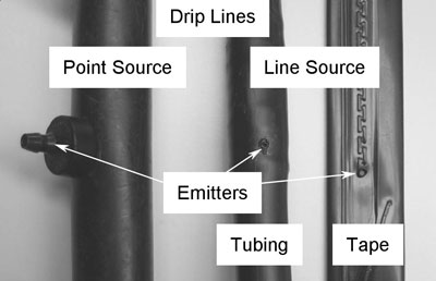
Figure 1. Examples of point source and line source emitters.
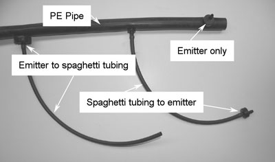
Figure 2. Spaghetti tubing for transporting water from point source emitter to plant.
Mainline valve
The mainline valve, the closest component to the water source, can be a gate valve (Figure 3), ball valve, or faucet, and is used to manually open and close water flow to the irrigation system. Secondary valves, either manual or electronic solenoid, are commonly used downstream of the main valve, but should not be used in place of the manual mainline valve.
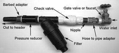
Figure 3. Example of components used in the mainline manifold of a high-pressure drip system.
Backflow prevention
A backflow prevention device is required in drip systems connected to a municipal or other potable water source. It prevents irrigation water from being siphoned back into, and potentially contaminating, the potable water if there is a sudden loss of pressure (e.g., the water main is closed, a major leak occurs in the main, etc.). In most urban areas, regulations specify what particular backflow prevention devices and installation procedures are required to legally comply with local building codes. Before designing or installing any irrigation system that will use domestic water, contact the local building inspector or water purveyor to ensure compliance with the correct backflow prevention requirements. A simple check valve (Figure 3) might be the only requirement to prevent backflow in some cases, but more fail-safe methods are usually required, such as anti-siphon valves or pressure vacuum breakers.
Filtration
A filter must be installed in the mainline (Figure 3) to prevent clogging of the emitters. It is an essential component of the system and should be used in all systems, regardless of the water source. There are two types of filters used in small drip systems: screen and disk (Figure 4). Screen filters have mesh sizes that range from about 50 to 200 (50 to 200 pores/inch, respectively). Disk filters consist of a stack of closely spaced disks, rather than screens, but their filtering capacity is still rated as a mesh size equivalency. A filter mesh size of about 150 is recommended for drip emitters that have flow rates between 0.5 and 10 gph (Drip Store, 2009). For the drip system to operate effectively, the filters must be regularly cleaned or flushed. If the water comes from an irrigation ditch and has a heavy silt load, filters may require cleaning after every irrigation or even during irrigation. Disk filters are better at filtering organic matter (e.g., algae cells) than screen filters and, based on experience at ASCF, seem to function better, with less clogging than screen filters. If sediments in the water are excessive, a sand filter or series of settling tanks may be required to pre-filter the water.
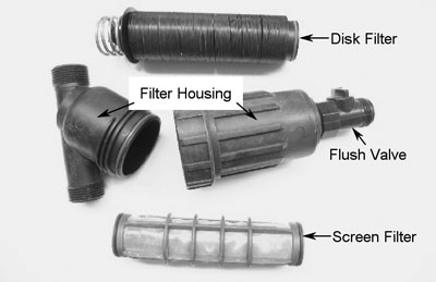
Figure 4. Example of types of filters used in small plot, drip-irrigation systems.
Pressure regulation
Drip irrigation systems are generally designed to operate in the pressure range of 10 to 30 pounds per square inch (psi), but domestic water is usually delivered to households at pressures above 30 psi. These higher pressures can blow out point source emitters and have an erosive effect on drip lines and other components. Therefore, a pressure reducer (or pressure regulator) should be used if the water delivered to the drip system comes from a domestic, or pump-driven, source. A pressure reducer (Figure 3) lowers the pressure to a specified level. A pressure regulator is more expensive than a pressure reducer, but the outlet pressure can be adjusted by turning a bolt on the regulator. For pressure reducers and regulators to function properly, there must be a minimum water pressure differential between the inlet and outlet of the reducer/regulator. This information should be available from the manufacturer or distributor.
When installing components of the manifold (Figure 3), it is important that the arrows stamped on check valves, pressure reducers, filters, and other components match the direction of water flow (i.e., the arrow points downstream).
Headers, end caps, footers, and flush valves
Downstream of the mainline, the header pipe distributes water directly to the drip laterals (Figure 5). Additional manual or electronic solenoid valves can be installed at various locations in the system to supply water to different zones or to individual laterals. Zoning is needed if available water flow is insufficient to satisfy the flow requirements of the entire system. Zoning is also used to separate plants with different water requirements so that each plant type receives the appropriate amount of water.
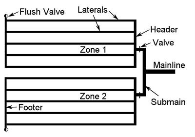
Figure 5. Example diagram of a simple, two-zone drip system.
Various methods can be used to cap the ends of the drip laterals, but whatever is used, it should allow for easy periodic flushing and draining of the laterals. In the crimping method, special "figure 8" fittings, or short pieces of 1- or 1 1/4-inch PE or PVC, can be used to hold a crimp at the end of 1/2-inch drip tubing. The ends of drip tape can be capped in the same manner by folding the tape at the end and holding the fold in place with a short (1-inch) piece of tape. Small plastic ball valves, which make lateral flushing and draining much easier than the crimp method, can also be used. They require clamping in high-pressure systems and are more costly than crimping.
In lieu of separate caps on each lateral, a footer pipe that connects the ends of all the drip laterals in a zone can be used (Figure 5). A single flush valve can then be installed at the lowest end of the footer to periodically flush and drain each zone. This option adds cost to the system since additional tubing and fittings are required, but it saves flushing time and helps equalize pressure throughout the zone.
Other fittings, Teflon tape, and clamps
Various plastic fittings (tees, elbows, couplers, etc.) are used to join drip lines. The appendages of barbed fittings (Figure 6) fit inside the drip lines and are held tightly to the drip line with stainless steel clamps (Figure 6). Compression fittings fit tightly to the outside of drip lines (Figure 6) and do not require clamps. Barbed fittings create a flow restriction at the pipe joint since they decrease the inside diameter of the pipe, but they are readily available at most hardware stores and are usually cheaper than compression fittings. In high-pressure systems, however, cost savings are neutralized by the additional expense of clamps required for the barbed fittings. Compression fittings do not restrict water flow, but they are not as readily available as barbed fittings and they are more difficult to disassemble once installed.
To prevent water leakage at threaded joints (nipples, filters, valves, etc.), all male threads should be wrapped (clockwise while facing threaded end) with a couple of layers of Teflon tape prior to assembly (Figure 6). Too much Teflon tape can create a leakage problem once the connectors are screwed together.
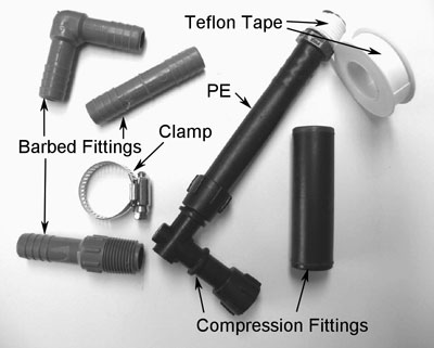
Figure 6. Examples of barbed and compression fittings, clamp, and Teflon tape.
Fertilizer injector
For vegetable gardening, a fertilizer injector is essential if the gardener's goal is high yields of good quality produce. Liquid fertilizers and other soluble chemicals are easily applied regularly into the water stream, which carries them to the soil around the base of each plant. With careful management, fertilizer efficiency is very high because it is applied frequently in low doses and there is no overspray or application to off-target areas. A simple, low-cost fertilizer injector (Figure 7) is suitable for small, high-pressure drip systems. If irrigation water has high levels of calcium (Ca), fertilizers with high phosphorus concentrations should be avoided because calcium phosphate (CaPO4) precipitates can form and clog emitters.
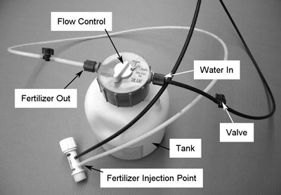
Figure 7. Example of a fertilizer injector for small drip systems.
Automation components
An electronic controller and solenoid valves, or in-line battery operated timers with built-in valves, can be used to automatically turn the water flow on and off at pre-programmed times. This automation is particularly useful if there are several different irrigation zones in the system and/or no one is available to manually control the system. Figure 8 shows an example of a four-zone manifold with electronic solenoid valves.
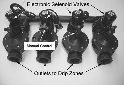
Figure 8. Four-zone manifold with electronic solenoid valves.
Other optional components
Air relief valves should be installed at high points in above-ground systems if the ground is excessively uneven or sloped (Burt and Styles, 1999), and in the above-ground manifolds of all buried systems. These valves are used to burp trapped air from the system. Water flow and pressure gauges, which can help indicate problems such as leaks or clogged filters or emitters, can also be installed in the water delivery lines of the system.
Drip Design Considerations
Pressure and flow rate
When designing a drip irrigation system, the required operating pressure of the emitter (specified by the manufacturer) and the flow rate of water in each section of distribution line or lateral that services the emitter must be considered. The greater the flow rate, which is determined by the sum of the flow rates of all outlets downstream of a particular pipe section, the greater the required inside diameter (ID) of that pipe section to minimize pressure differences between outlets caused by friction. Unlike sprinkler or flood irrigation systems, which require large ID piping (e.g., 2- to 10-inch) to satisfy the high gallon per minute (gpm) flow rates of the outlets, drip line IDs are usually less than 1 inch since flow rates are very low (usually measured in gph). For example, the flow rate of one brass Rainbird model 30H impact sprinkler operating at 50 psi is equivalent to the flow rate of more than 500 1-gph emitters (8.3 gpm).
Table 1 shows the relationship between pressure loss and flow rate for different PE pipe sizes commonly used in drip irrigation systems (Hunter Industries, 2001). Note that the nominal (in name only) size of pipe does not necessarily equal the pipe's ID. In fact, as shown in the top row of Table 1, there are three different IDs associated with nominal 1/2-inch PE pipe available from this manufacturer: 0.520, 0.600, and 0.620 inch. It is very important to identify the actual ID of the nominal 1/2-inch pipe that is being used for the drip system for a couple of reasons. First, the pressure loss due to friction per 100 feet of the 0.520-inch ID pipe is about double that of the 0.600-inch ID pipe and about 2.3 to 2.4 times that of the 0.620-inch ID pipe (Table 1). While the 0.520-inch ID may be more than adequate for short drip laterals with low flow rates (i.e., less than 200 feet and 60 gph, respectively), the larger ID sizes should be used for longer laterals with higher flow rates. Second, compression or barbed fittings are generally not interchangeable between the different (nominal) 1/2-inch pipe sizes. If the actual ID and outside diameter (OD) are known, the proper fittings can be obtained for constructing a new system or for repairing an existing system.
Table 1. Pressure Loss Per 100 Feet for Selected Sizes of Polyethylene (PE) Pipe (Pepco Products) at Various Flow Ratesa
| PE pipe less than 3/8 inch | PE pipe greater than 3/8 inch | ||||||||||
|---|---|---|---|---|---|---|---|---|---|---|---|
| Nominal size | 1/4 inch | 5/16 inch | 3/8 inch | 1/2 inch | 1/2 inch | 1/2 inch | 5/8 inch | 3/4 inch | 1 inch | 1 1/4 inches | |
| Pipe ID (inch) | 0.170 | 0.250 | 0.375 | 0.520 | 0.600 | 0.620 | 0.720 | 0.830 | 1.060 | 1.39 | |
| Pipe OD (inch) | 0.250 | 0.307 | 0.455 | 0.620 | 0.700 | 0.710 | 0.830 | 0.940 | 1.200 | 1.55 | |
| Wall thickness (inch) | 0.040 | 0.028 | 0.040 | 0.150 | 0.050 | 0.045 | 0.055 | 0.055 | 0.070 | 0.080 | |
| Flow (gph) | Pressure loss per 100 feet (psi) | Flow (gph) | Pressure loss per 100 feet (psi) | ||||||||
| 2.0 | 0.49 | 0.08 | 0.01 | 30 | 0.32 | 0.16 | 0.14 | 0.07 | 0.03 | 0.01 | 0 |
| 2.5 | 0.75 | 0.11 | 0.02 | 45 | 0.68 | 0.34 | 0.29 | 0.14 | 0.07 | 0.02 | 0.01 |
| 3.0 | 1.05 | 0.16 | 0.02 | 60 | 1.17 | 0.58 | 0.50 | 0.24 | 0.12 | 0.04 | 0.01 |
| 3.5 | 1.39 | 0.21 | 0.03 | 75 | 1.76 | 0.88 | 0.75 | 0.36 | 0.18 | 0.06 | 0.01 |
| 4.0 | 1.78 | 0.27 | 0.04 | 90 | 2.47 | 1.23 | 1.05 | 0.51 | 0.25 | 0.08 | 0.02 |
| 4.5 | 2.22 | 0.34 | 0.05 | 105 | 3.29 | 1.64 | 1.40 | 0.67 | 0.34 | 0.10 | 0.03 |
| 5.0 | 2.69 | 0.41 | 0.06 | 120 | 4.21 | 2.10 | 1.79 | 0.86 | 0.43 | 0.13 | 0.04 |
| 6.0 | 3.78 | 0.58 | 0.08 | 135 | 5.23 | 2.61 | 2.22 | 1.07 | 0.54 | 0.16 | 0.04 |
| 7 | 5.03 | 0.77 | 0.11 | 150 | 6.36 | 3.17 | 2.70 | 1.31 | 0.65 | 0.20 | 0.05 |
| 8 | 6.44 | 0.99 | 0.14 | 165 | 7.59 | 3.78 | 3.22 | 1.56 | 0.78 | 0.24 | 0.06 |
| 9 | 8.00 | 1.23 | 0.17 | 180 | 8.91 | 4.44 | 3.79 | 1.83 | 0.92 | 0.28 | 0.07 |
| 10 | 9.73 | 1.49 | 0.21 | 195 | 5.15 | 4.39 | 2.12 | 1.06 | 0.32 | 0.09 | |
| 12 | 2.09 | 0.29 | 210 | 5.91 | 5.04 | 2.43 | 1.22 | 0.37 | 0.10 | ||
| 14 | 2.78 | 0.39 | 225 | 6.72 | 5.73 | 2.77 | 1.38 | 0.42 | 0.11 | ||
| 16 | 3.56 | 0.49 | 240 | 7.57 | 6.45 | 3.12 | 1.56 | 0.47 | 0.13 | ||
| 18 | 4.42 | 0.62 | 270 | 9.41 | 8.03 | 3.88 | 1.94 | 0.59 | 0.16 | ||
| 20 | 5.38 | 0.75 | 300 | 9.76 | 4.71 | 2.36 | 0.72 | 0.19 | |||
| 22 | 6.42 | 0.89 | 330 | 5.62 | 2.81 | 0.86 | 0.23 | ||||
| 24 | 7.54 | 1.05 | 360 | 6.61 | 3.31 | 1.01 | 0.27 | ||||
| 26 | 8.74 | 1.22 | 390 | 3.84 | 1.17 | 0.31 | |||||
| 28 | 10.03 | 1.39 | 420 | 4.40 | 1.34 | 0.36 | |||||
| 30 | 1.58 | 450 | 5.00 | 1.52 | 0.41 | ||||||
| a Table adapted from Handbook of Technical Irrigation Information, produced by Hunter Industries | |||||||||||
In the absence of a pump, static pressure (pressure when no water is flowing) at any point in a drip system is created by the height of the water surface above the emitter. Pressure is measured in psi, and each 2.31 feet of water (head) above an emitter or other point in the irrigation system provides 1 psi of static pressure at that point. On a sloped or uneven field, static pressure changes with elevation. In a perfectly level field, the difference in dynamic pressure (pressure when water is flowing) from one point to another along the drip line will be due to friction only (Table 1). Ideally, drip laterals should be kept as short as practical to minimize pressure loss due to friction, and should be laid slightly downslope (from header to footer) on sloped plots to help neutralize friction loss with pressure gain created by the increased head from the water surface to the downslope emitters. On very steep slopes, it is best to lay the drip lines along the contour of the slopes rather than upslope or downslope to avoid excessive pressure variability between emitters. Pressure compensating (PC) emitters are designed to emit the same flow rate within a wide range of pressures (Figure 9) and should be used on terrain that is excessively undulated or uneven.
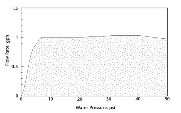
Figure 9. Example of the flow rate of a pressure compensating (PC) emitter at different water pressures.
Another suggestion when obtaining components for a point source drip system is to use utility or irrigation grade PE pipe rather than drinking water grade. Drinking water grade PE is more expensive than utility grade PE, and its greater wall thickness makes fittings and point source emitters much more difficult to install.
Advantages of Drip Over Sprinkler or Flood Irrigation
Improved water efficiency
Early in the growing season, water losses through direct soil surface evaporation are less with drip irrigation, which wets only a small area around the base of each plant, than with sprinkler or flood irrigation, which wets the entire soil surface. Unlike sprinkler or flood irrigation, surface runoff of water is virtually non-existent in drip irrigation. Water application uniformity, a measure of irrigation efficiency, is usually much better in drip irrigation than in sprinkler or flood irrigation because drip is not affected by wind (as in sprinkler irrigation) and water is not applied down furrows between rows (as in flood irrigation). Since each plant theoretically receives the same volume of water in a well-designed drip system, plant growth and yield should be relatively uniform over the entire irrigated area.
Weed and disease control
A major advantage of drip irrigation over other methods in the dry climate of the Southwest is reduced weed growth between crop rows. When the entire soil surface is continuously wetted, as in sprinkler or flood irrigation, weed seeds in the soil between the rows continue to germinate throughout the growing season. Even if preplant herbicides are used, their effectiveness may be diminished if the active ingredients are diluted or leached by excessive sprinkler or flood irrigation. Because herbicide use and hand hoeing are reduced with drip irrigation, money spent on weed control is saved and crop yield and quality are not as adversely affected by weed competition as they can be in sprinkler and flood irrigation. The potential for foliar diseases is also reduced compared to sprinkler irrigation since the leaves and stems of the crop are not being wetted.
Fertilization
As mentioned previously, liquid fertilizers (water soluble, e.g., all-purpose, 32-0-0, etc.) can be injected directly into the irrigation stream and applied to the soil right at the base of each plant. It can be applied frequently and at very low doses to "spoon feed" the plants throughout the growing season. With careful management, fertilizer losses are minimal and fertilizer efficiency is very high.
Versatility and conformity
The small-diameter PE pipe used in drip irrigation is flexible and can easily conform to the garden or landscape configuration and topography. Crops do not need to be planted in straight rows, but can instead be planted along contours of the land. With point source systems, plant spacing can be highly variable, and the number and flow rates of emitters can be selected to satisfy the specific water requirements of each plant within an irrigation zone or landscape.
Disadvantages of Drip Over Flood or Sprinkler Irrigation
Irrigation management challenges
Because of the small, but localized, volumes of water applied to plants under drip irrigation, the water must be applied frequently (every day to every other day for annual vegetable crops, and once or twice per week for deeper rooted perennials) and for relatively short durations (a few hours or less) depending on the crop, the crop's growth stage, the absorptive capacity of the soil, and the flow rates of the emitters. While this may not be a limiting factor when using a municipal, water-on-demand system, particularly if the drip system is automated, it can be problematic for irrigators using water from canals, ditches, and acequias where water availability may be restricted by specific, predetermined schedules set by the water purveyor or district. If water can only be obtained once per week for a 24-hour period, for example, drip irrigation management becomes very difficult unless water can be stored in a pond or tank for use on demand.
Another common problem with drip irrigation is the perception by irrigators accustomed to sprinkler or flood irrigation that not enough water is being applied. There can be a tendency to apply more water than required for adequate plant growth to make up for the perceived water deficit. This excess water, along with essential, readily soluble nutrients in the soil (such as nitrogen and potassium) may be lost from the plant root zone through deep percolation. This results in water and fertilizer waste and potential reduction in crop yield.
In areas with saline soil or water, salts can reduce soil quality and adversely affect plant growth by accumulating at the perimeter of the area wetted by emitters (Burt and Styles, 1999). Periodic sprinkler irrigations may be required if natural precipitation is insufficient to leach this accumulated salt into the soil below the plant root zone.
Contraction and expansion of PE laterals
Since PE drip line is flexible, it contracts and expands with temperature changes. Consequently, it may be necessary to lay out the drip laterals and fill them with cool irrigation water either before planting (with line source systems) or before installing emitters (with point source systems). This is of particular concern if the drip lines are very long (150 feet or more) and the emitters are widely spaced (greater than 24 inches). If the lines are laid out when they are warm, which is preferable because they are more pliable and easier to work with, they will be expanded. If transplants or seeds are planted next to an emitter on a warm, expanded line, water may not be applied directly to the plants or seeds when it is filled with cool water and it contracts. Because of this, line source drip lines should be filled with water and run for a while to create wet spots where the transplants or seeds should be planted. With a point source drip line, planting can be done before laying out the PE line next to the plants, but the line should be filled with water prior to installing the emitters so their placement will be in close proximity to the plants. If the chosen point source emitters can accommodate spaghetti tubing, it can be used to distribute water from the emitter outlet closer to the base of the plant if necessary (Figure 2).
Damage to components
The small plastic components of drip systems are fragile and are easily damaged by equipment, animals, or humans. Cheap, thin-walled drip tape and other exposed components can deteriorate when exposed to weathering and the ultraviolet rays of the sun. In subsurface drip systems, buried lines can incur significant damage from pocket gophers and other burrowing rodents. These problems can be overcome by selecting high-quality materials, by covering above-ground components with mulch, and by avoiding subsurface drip where burrowing rodents are common.
Water quality and emitter clogging
Clogging of drip emitters by particulate matter can usually be prevented with proper filtration and lateral flushing. If the irrigation water is high in calcium and bicarbonates, chemical clogging by precipitates of calcium carbonate (CaCO3) may occur. Additionally, if the water source is a pond or open irrigation canal, algae or other organic material may clog filters and emitters. Chemical clogging can be prevented by adding an acid (e.g., vinegar) to the water, while adding chlorine (e.g., bleach) can help remediate biological clogging.
Economic considerations
Considering the initial costs for components and installation, drip irrigation is more expensive than flood irrigation (Burt and Styles, 1999), and drip upkeep costs may be greater than upkeep costs for sprinkler systems. Over time, however, if components are well maintained and used for many years, these higher initial costs will be recovered by reduced labor costs, reduced inputs of fertilizers and pesticides, higher quality and yields of produce, and lower water use compared to flood or sprinkler irrigation.
Low-Pressure Drip
In this paper, low-pressure drip irrigation will be defined as water supplied through piping and emitters from an elevated reservoir (e.g., tank, pond, irrigation ditch) to a garden or landscape at a head of less than 20 feet, or 8.7 psi of pressure (20/2.31), to the emitters.
Advantages of low-pressure drip compared to high-pressure drip
Only two primary components are required in the mainline manifold of a low-pressure, gravity system: a valve and a filter (Figure 10). Since the water reservoir surface is elevated above the emitters and there is a break between water inflow and outflow, a backflow prevention device is not required. Pressure is already low, so a pressure regulator is not needed, and since fertilizer can be added directly to the elevated tank, a fertilizer injector is not required. Unlike high-pressure systems, which require tight-fitting compression fittings or clamped barbed fittings to prevent blowouts and leaks, a friction fit between PE tubing and barbed fittings is usually sufficient to hold connections together in a low-pressure system. Short (1-inch) pieces of an old 1/2- or 5/8-inch garden hose, rather than clamps or specialized fittings, can sometimes be used to clamp drip tape to barbed fittings.
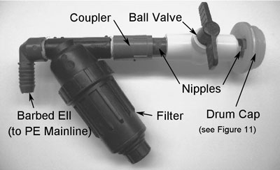
Figure 10. Example of components used in the manifold of a low pressure drip system.
Disadvantages of low-pressure drip compared to high-pressure drip
One major disadvantage of a low-pressure system is that emitter flow rates are lower than those specified by the manufacturer at their recommended operating pressure (usually greater than 10 psi). Consequently, on-site measurements are required to identify the actual flow rate of emitters and to determine the application uniformity (how evenly water is applied to all plants) at these lower pressures.
Determining emitter flow rate and application uniformity. Average emitter flow rate and system application uniformity (AU) can be determined by placing a small container (e.g., tuna can) into depressions dug into the soil under selected emitters along laterals and recording the volume of water caught in each container during a specified period of time. Each lateral should be of the desired length (preferably less than 100 feet), and in the case of point source laterals, all emitters of the zone should be installed. If all laterals fed by a header are similar (same type, ID, length, flow rate, etc.), the irrigated area is level, and the header is of sufficient size to minimize friction loss between laterals (Table 1), measurements from one lateral should represent measurements from all laterals fed by the header. Measurements should be taken from emitters near the header, midway between the header and footer, and close to the footer (or flush end) of the farthest lateral from the mainline to determine flow rate variability between emitters. While it is preferable to measure the volume of water caught in each can with a graduated cylinder that has a milliliter (ml) scale, a tablespoon or small measuring cup with a fluid ounce scale can be used. The following conversion factors and equation can be used to convert flow rate from ml/second to gallons per hour (gph):
Conversions:
1 fluid ounce = 30 ml
1 tablespoon = 0.5 fluid ounce (or 15 ml)
1 gallon = 3,785 ml
Equation: Flow rate (gph) = (volume caught [ml] Ö time [seconds]) x 0.95
As a general rule, emitter flow rates taken from different emitters should not differ by more than 20%. If it appears that emitter flow rate is decreasing with increased distance from the header, laterals may be too long and should be shortened. If plant rows to be irrigated with low pressure are more than 100 feet long, AU may be improved by positioning the header across the center of the garden (perpendicular to the rows) and connecting the laterals to the header so they distribute water down the rows in both directions from the central header.
Low-pressure emitters
An experiment was undertaken at ASCF in 2010 to determine which components might be suitable for use in low-pressure, rainwater catchment systems. Flow rates were measured for seventeen different point source emitters, two line source tubings, and one (line source) drip tape at a low pressure of 2.5 psi (6 feet of head). The average flow rates and AUs of one line source drip tape, one line source drip tubing, and five different models of point source emitters are shown in Table 2. Each flow rate value (column 3) represents the mean of several measurements taken from emitters located at various distances along replicated 50-foot and 100-foot laterals. The uniformity (column 2) is expressed as 1 - cv (coefficient of variability), where cv is the standard deviation divided by the average of all measurements for a given emitter model. The closer uniformity is to 1, the less difference there is in the flow rate between emitters.
Table 2 shows only those emitters (or lines) for which uniformity was greater than 0.85. The measured flow rate is also expressed as a percentage (% MSFR, column 4) of the manufacturer-specified flow rate (MSFR, column 5) at the recommended pressure range. The manufacturer's recommended minimum pressure (MRMP) is shown in column 6. Average flow rate per emitter ranged from 0.104 gph for the drip tape to 1.174 gph for the D002 emitter (39% and 58.7% of the MSFR of 0.27 and 2.0 gph, respectively, at pressures greater than 10 psi). The drip tape and the emitter D012 provided the best application uniformity of all emitters tested (0.958 and 0.957, respectively), but the flow rates were very low (0.104 and 0.336 gph).
Table 2. Measured Application Uniformity, Flow Rate, and Percent of Manufacturer's
Specified Flow Rate at Recommended Pressure of Five Point Source and Two Line
Source Emitters When Operated at Low Pressure (2.5 psi)
|
Emitter Model |
Uniformity |
Flow Rate (gph) | MRMPd,e | ||
|---|---|---|---|---|---|
| Measured | % MSFRc | MSFR | psi | ||
| D012 | 0.957 | 0.336 | 33.6 | 1.0 | 20 |
| D006 | 0.940 | 0.519 | 51.9 | 1.0 | ns |
| D023 | 0.913 | 0.991 | 24.8 | 4.0 | 20 |
| D002 | 0.894 | 1.174 | 58.7 | 2.0 | ns |
| D013 | 0.871 | 0.723 | 36.1 | 2.0 | 20 |
| Drip Tape (Ro-Drip) |
0.958 | 0.104 | 39.0 | 0.27 | 10 |
| Drip Tube (0.600") | 0.940 | 0.315 | 31.5 | 1.0 | 10 |
|
a Item number at The Drip Store (www.dripirrigation.com). Actual model number may vary from that of the manufacturer or between distributors. b cv - coefficient of variability (mean/standard deviation) c MSFR - manufacturer's specified flow rate at recommended pressures d MRMP - manufacturer's recommended minimum pressure e ns - not specified, but minimum recommended operating pressure assumed to be 10 psi |
|||||
It is important to identify the actual emitter flow rates and the system AU under these low-pressure conditions so irrigations can be scheduled effectively and efficiently. If the drip system cannot provide the maximum daily water requirements of the plants being irrigated, plant growth and yields (vegetable crops) or plant quality (landscape plants) may be unacceptably reduced.
Irrigation Scheduling
Crop water use or evapotranspiration
Plant water requirements are directly related to the plant's live leaf area and daily weather conditions (Allen et al., 1998). The greater the leaf area, the hotter the air temperature, the higher the wind speed, the greater the sunlight, and the drier the air (low relative humidity), the more water will be required to replace plant water use or evapotranspiration (ET). In large agricultural or turfgrass fields, crop ET (ETc) is usually expressed in depth units (inches or mm). Crop ET is estimated by multiplying a reference ET (ETr), which is calculated with weather data, by an adjustment factor called a crop coefficient (Kc) to account for variables such as plant species and plant growth stage (height or canopy area that causes actual ETc to deviate from the calculated ETr). Early in the growing season, for example, plants are small and ETc is low (e.g., 0.1 inch/day). Daily ETr, on the other hand, is relatively low (e.g., 0.3 inch/day) compared to midsummer, but is much higher than ETc, so the ratio of ETc to ETr (Kc) is relatively low (ETc/ETr = 0.10/0.30 = 0.33). In late spring and into early summer, ETc increases rapidly as plant size and leaf area increase and reaches a peak value (e.g., 0.4 inch/day) in midsummer. Average daily ETr also increases with the longer and hotter days (e.g., to 0.4 inch/day in midsummer), but does not increase at the same rate as ETc. As the crop canopy closes and completely shades the ground, daily ETc may equal or exceed ETr, in which case Kc may equal or exceed 1.0 (e.g., ETc/ETr = 0.45/0.40 = 1.125).
Drip irrigation requirement
Seasonal crop coefficient (Kc) curves have been formulated for many different crops (Allen et al., 1998), and if appropriate weather data are available to calculate ETr, they can be used to estimate the water use of these crops when grown in large monocultures. A modification of the technique (Equation 1) can be used to estimate the irrigation requirement (IR) of individual plants in small, drip-irrigated vegetable gardens and landscapes (Smeal et al., 2010). To calculate IR, measurements of the plant's canopy diameter (D) and ETr (Table 3), which vary during the growing season, are multiplied by an adjustment factor (AF) and a constant (0.49) that converts D to plant canopy area (circular ft2) and IR from inches to gallons (Equation 1). To prevent over-irrigation, effective precipitation (inches) between irrigations is subtracted from ETr (Equation 1). To calculate effective precipitation (EP), measured rainfall events less than 0.2 inch are ignored, and only 75% (0.75) of the amounts in excess of 0.2 inch are considered (Farmwest.com, 2004). To help prevent under-irrigation of plants, IR is adjusted upward by the AU or irrigation efficiency (IE) to help compensate for uneven flow rates of emitters. Until transplants are fully established, IE is set to 0.5 to wet a large area for plant root development. After the plants show signs of new growth, IE should be set to the AU value if known. If unknown but all emitters appear to be wetting an equal area around the base of all plants, IE can be set to 0.9.
Table 3. Average Daily Reference ET (ETr) Values for Two-Week Periods During
the Growing Season at NMSU's Agricultural Science Center at Farmingtona
| Month |
Days of |
Avg. Daily |
Month |
Days of Month |
Avg. Daily |
|---|---|---|---|---|---|
| March | 1-15 | 0.17 | July | 1-15 | 0.38 |
| 16-31 | 0.21 | 16-31 | 0.34 | ||
| April | 1-15 | 0.24 | August | 1-15 | 0.32 |
| 16-30 | 0.28 | 16-31 | 0.29 | ||
| May | 1-15 | 0.32 | September | 1-15 | 0.26 |
| 16-31 | 0.35 | 16-30 | 0.24 | ||
| June | 1-15 | 0.38 | October | 1-15 | 0.21 |
| 16-30 | 0.40 | 16-31 | 0.16 | ||
| a The average ETr values shown between May 15 and September 15 are fairly typical for most of New Mexico north of Los Lunas, but can vary significantly with local microclimatic conditions. | |||||
Equation 1: Calculating the drip irrigation requirement of an individual plant
IR = (ETr - EP) x AF x D2 x 0.49 / IE
Where:
IR = irrigation requirement of the plant in gallons per day
ETr = reference ET/day in inches (from Table 3 for Northern NM)
EP = 0.75 multiplied by the sum of rainfall events greater than 0.2 inch, minus 0.2 inch per event
AF = adjustment factor for the plant (see Adjustment Factors section in this paper)
D = measured plant canopy diameter in feet
0.49 = constant that converts inches to gallons and plant canopy diameter to canopy area
IE = irrigation efficiency = application uniformity (1 Ð cv)
Adjustment factors (AF)
Experiments conducted at ASCF have shown that AF for use in Equation 1 varies significantly between different plant species. In a xeriscape demonstration and research garden at the center, for example, AF values range from less than 0.1 for very drought-tolerant, native New Mexico species such as desert willow (Chilopsis linearis) to greater than 1.0 for the purple coneflower (Echinacea purpurea), a species native to wetter areas of the U.S. north and east of New Mexico. A list of the AF values from more than 90 species in the garden is available from the ASCF website (Smeal et al., 2010). In drip-irrigated vegetable research conducted during the past five years, AF values that provided maximum yields of chile peppers, tomatoes, and sweet corn averaged 0.80, 0.70, and 0.90, respectively. While future research studies at the ASCF may identify unique AF values for other crops, a baseline value of 0.8 will probably suffice for most vegetable crops. If the plants appear to be receiving insufficient or excessive water, AF can be adjusted up or down slightly as conditions warrant.
Plant canopy areas
Equation 1 is used to estimate the IR of individual plants when there is incomplete plant canopy coverage (i.e., the plant canopy does not completely shade the ground). A yardstick or tape measure is used to measure D during the season, and it is inserted into Equation 1 to calculate plant IR for that particular day. Equation 2 should be used to estimate the IR per plant if and when the ground surface is completely shaded by the plant canopy. In this formula, canopy area (CA) per plant is considered equal to the row spacing (ft) multiplied by the plant spacing (ft) within the row. For example, if tomatoes are planted in rows 3 feet apart and the plants are 2 feet apart in the row, CA at full canopy coverage will be 6 square feet per plant (3 ft x 2 ft).
Equation 2: Calculating the irrigation requirement per plant of row crops when the mature canopy completely shades the ground
IR = (ETr - EP) x AF x CA x 0.623 / IE
Where:
IR = irrigation requirement of the specific plant in gallons per plant (gpp)
ETr = reference ET in inches (from Table 3 for Northern NM)
EP = 0.75 multiplied by the sum of rainfall events greater than 0.2 inch, minus 0.2 inch per event
AF = adjustment factor for the plant
CA = plant canopy area in ft2 (row spacing x plant spacing, in ft)
0.623 = constant that converts inches/ft2 to gallons
IE = irrigation efficiency = application uniformity (1 Ð cv)
System capacity and maximum daily irrigation requirement
In planning a drip-irrigated garden or landscape, sufficient water should be available to satisfy IR for all plants in the garden during midsummer, the peak water requirement (PWR) period. Because of low flow rates in drip irrigation, it is likely that plenty of water will be available to satisfy the PWR of a fairly large garden if the water is from a pressurized, municipal source. If you are relying on a limited volume of water (e.g., rainwater catchment tank), however, it is essential to accurately estimate PWR of the planned garden and volume of water that will be available to satisfy PWR. Equations 1 and 2, along with estimates of each plant's maximum CA, can be used to estimate PWR for each plant. Individual PWR can then be summed to get an estimate of total PWR of the landscape or garden (Examples 1 and 2).
Example 1: Calculating the peak water requirement of a theoretical xeriscape
Suppose you are planning a small xeriscape that will consist of the following plants:
- Five shrubs, each with a mature canopy diameter (D) of 5 feet
- The AF for two of the shrubs is 0.40 (shrub 1)
- The AF for three of the shrubs is 0.25 (shrub 2)
- Two trees with a mature D of 12 feet per tree
- The AF of one tree is 0.60 (tree 1)
- The AF of the other tree is 0.10 (tree 2)
- Twenty smaller perennials, each with an average maximum D of 2 feet
- The AF of five of the plants is 0.15, plant type 1 (P-1)
- The AF of ten of the plants is 0.30, plant type 2 (P-2)
- The AF of five of the plants is 0.50, plant type 3 (P-3)
To solve:
- Set up a table and insert the values of the parameters needed to solve IR for each plant type (Table 4). Assume the worst-case scenario of maximum ETr (0.40 inch/day) and no rain. In this example, we'll set IE (or AU) to 0.9.
- Calculate the IR per plant (column 5 of Table 4) using Equation 1.
- Multiply IR per plant by the number of plants (column 6) of the same type.
- Add the IRs of all plants (column 7).
In Example 1, the average daily PWR in midsummer for the entire landscape is about 36 gallons per day (Table 4) or 252 gallons per week. Note that Tree 1, which has an AF of 0.6, uses more than half the PWR for the entire landscape. If the anticipated available water is lower than that required to satisfy the PWR of the xeriscape, replacing Tree 1 with a desert willow, or something similar with a lower AF, would have the greatest impact on water savings.
Table 4. List of Parameters and Calculation of Peak Water Requirementa for a Theoretical Xeriscape Using Equation 1
| Plant Species | D (feet) |
AF | D2 (feet) |
Equation 1: IR/Plant = ETr x AF x D2 x 0.49 / IE (gal/day) |
No. of Plants | IR (all plants) (gal/day) |
|---|---|---|---|---|---|---|
| Shrub 1 | 5 | 0.40 | 25 | 0.4 x 0.4 x 25 x 0.49 / 0.9 = 2.18 | 2 | 4.36 |
| Shrub 2 | 5 | 0.25 | 25 | 0.4 x 0.25 x 25 x 0.49 / 0.9 = 1.36 | 3 | 4.08 |
| Tree 1 | 12 | 0.60 | 144 | 0.4 x 0.6 x 144 x 0.49 / 0.9 = 18.82 | 1 | 18.82 |
| Tree 2 | 12 | 0.10 | 144 | 0.4 x 0.1 x 144 x 0.49 / 0.9 = 3.14 | 1 | 3.14 |
| P-1 | 2 | 0.15 | 4 | 0.4 x 0.15 x 4 x 0.49 / 0.9 = 0.13 | 5 | 0.65 |
| P-2 | 2 | 0.30 | 4 | 0.4 x 0.3 x 4 x 0.49 / 0.9 = 0.26 | 10 | 2.60 |
| P-3 | 2 | 0.50 | 4 | 0.4 x 0.5 x 4 x 0.49 /0 .9 = 0.44 | 5 | 2.20 |
| Total IR for landscape (gal/day) | 35.85 | |||||
| a This same procedure is used for estimating the IR per plant throughout the season, except actual measured D and ETr for the day (minus EP) are used instead of estimated maximums. | ||||||
Example 2: Calculating the peak water requirements of a vegetable garden
Suppose you are planning a vegetable garden consisting of chile peppers, tomatoes, and sweet corn that will be planted in rows. Row spacing for all crops will be 3 feet, and the in-row spacing will be 3 feet for tomatoes and 1 foot for both the peppers and sweet corn. Because growth rates and water requirements will differ between crops, you split the garden into three zones. Each zone consists of five 50-foot-long rows, for a total area per zone of 750 square feet (5 rows x 3 ft x 50 ft). The tomato and sweet corn canopies will completely shade the ground in midsummer, but the diameter of each chile plant will be only 18 inches, or 1.5 feet, and they were planted in rows 3 feet apart to allow room for multiple hand harvests. Assume no rain and an IE (or AU) of 0.90.
To solve:
- Construct a table (Table 5) and enter the appropriate values to compute PWR (or IR).
- Since the chile canopy will not completely shade the ground, use Equation 1 with the maximum D (assume 1.5 ft) and AF for chile (0.80) to calculate the PWR (or IR at peak of summer) per plant:
- IR for chile: Equation 1: IR = (ETr - EP) x AF x D2 x 0.49 / IE = (0.4 - 0) x 0.80 x (1.5 x 1.5) x 0.49 / 0.90 = 0.39 gal/plant/day
- Since the sweet corn and tomato canopies will completely shade the ground in midsummer, use Equation 2 with either the maximum CA per plant (1 ft x 3 ft = 3 ft2 for the corn, and 3 ft x 3 ft = 9 ft2 for the tomatoes) or the entire CA of each zone (5 rows x 3 ft spacing x 50 ft long = 750 ft2) and AFs of 0.90 and 0.70 for the corn and tomatoes, respectively, to calculate the PWR of each zone. Whichever is chosen, the number of plants in each zone will need to be known to calculate the PWR per plant (i.e., total zone area/CA per plant).
IR for sweet corn and tomato: Equation 2: IR = (ETr - EP) x AF x CA x 0.623 / IE =
(0.40 - 0) x 0.90 x 750 x 0.623 / 0.90 = 186.9 gal/day for all sweet corn plants
(0.40 - 0) x 0.70 x 750 x 0.623 / 0.90 = 145.4 gal/day for all tomato plants
The total daily PWR of the garden is about 430 gallons (Table 5). Using the PWR, you can estimate how many plants of each type can be adequately watered during midsummer. If you have less than 430 gallons of water per day available, you'll need to reduce the quantity of plants so that PWR of the remaining plants can be satisfied to avoid plant water stress and yield reductions.
Table 5. Estimated Plant Parameters and Calculated Peak Water Requirementa of the
Example 2 Vegetable Garden
| Vegetable Crop |
D ft |
CA ft2 |
AF inch |
ETr/day | No. of Plants |
IR/plant gal/day |
Total IR gal/day |
|---|---|---|---|---|---|---|---|
| Chile | 1.5 | n/a | 0.80 | 0.4 | 250 | 0.39 | 97.5 |
| Sweet Corn | n/a | 750 | 0.90 | 0.4 | 250b | 0.75c | 186.9 |
| Tomatoes | n/a | 750 | 0.70 | 0.4 | 83b | 1.75c | 145.4 |
| Estimated daily peak water requirement of entire garden in summer | 429.8 | ||||||
|
a This same procedure is used for estimating the IR per plant throughout the season, except actual measured D and ETr for the day (minus EP) are used instead of estimated maximums. b 750 ft2 Ö (row spacing x plant spacing in ft) c Total IR Ö number of plants |
|||||||
Irrigation duration and frequency
To determine how long you'll need to run the system to satisfy PWR, divide the PWR per plant by the emitter flow rate. Suppose you are using emitter D012 with a flow rate of 0.34 gph (Table 2) to irrigate the vegetable crops in Table 5 during the midsummer PWR period. If watering every day, you would need to irrigate the chile, corn, and tomatoes for 1.15 (0.39 / 0.34), 2.21 (0.75 / 0.34), and 5.15 (1.75 / 0.34) hours, respectively. Plants do not necessarily require daily irrigations. In studies conducted at ASCF, we irrigated the xeriscape plants once per week and the vegetable garden plants every other day. If irrigating at this frequency, the daily IR and irrigation duration would be multiplied by seven for xeriscape plants and by two for the vegetable plants.
If you're using a municipal water source, you can use IR or PWR to estimate the approximate cost of irrigating the garden each month or billing period. Farmington (2010), for example, uses a bracketed water rate structure in which the cost per unit (1,000 gal) of water used below 7 units is $2.09, while the cost per unit between 7 and 20 units is $2.61. If the average monthly non-irrigation water is about 5,000 gal/month, the total additional cost of irrigation water in July, assuming peak water use every day (about 12,000 gal), would be about $30 (2 units at $2.09 and 10 units at $2.61) for the garden in Example 2 if no rain occurs.
In a rainwater catchment system, the volume of water potentially available for irrigation or other purposes depends on the area of the runoff collection surface (e.g., roof) and the depth of irrigation. It takes 0.623 gallons of water to fill a 1-square-foot area to a depth of one inch. Therefore, 0.623 x runoff area (ft2) x precipitation (inch) = potential gallons collected. For example, if the total annual precipitation in the Farmington area (8.2 inches) was collected from a 24 by 40 foot rooftop, it would yield about 4,900 gallons (0.623 x 24 ft x 40 ft x 8.2 in.).
Example of Gravity Irrigation System
Elevated, 55-gallon plastic drums, mounted on fabricated metal stands or inexpensive stands consisting of four 8-foot-long steel T posts and baling wire, were used to irrigate several vegetable garden plots during experiments conducted at ASCF (Figure 11). An opening was cut into the side of the barrel (top of barrel once mounted on stand) for easy cleaning, adding water and fertilizer, or other access needs (Figure 12). The water level in the drum was maintained using pressurized water that flowed through a hose inlet assembly and float valve mounted at the upper barrel cap of the drum (Figure 12). While this float assembly was used for convenience in our experiments, it is not required in rainwater catchment systems or drums that will be filled by hand using buckets or a hose. In our studies, the water level was maintained at approximately 6 feet above the soil surface, which provided about 2.5 psi of pressure (6/2.31) at the emitters.
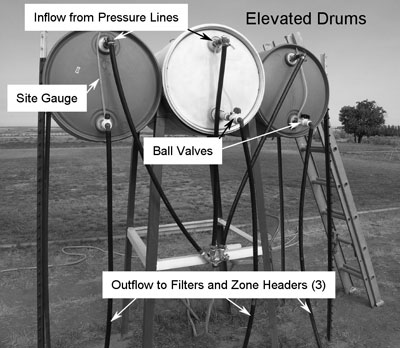
Figure 11. Elevated tanks used to provide water at low pressure to drip irrigation systems.
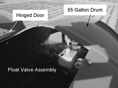
Figure 12. Hinged door cut into tank and float valve.
A list of the components with their approximate costs to construct a small gravity feed drip system using a 55-gal plastic drum is shown in Table 6. In this system, the drum is mounted on wires strung between four steel fence posts. A door is cut into the upper-facing side of the drum to gain access for adding water or fertilizer. A 3/4-inch PE main line with a ball valve and filter installed controls water flow from the bottom outlet of the drum to a 3/4-inch PE header. The laterals are 1/2-inch PE, and three different options are illustrated: 1) line source drip tubing, 2) line source drip tape, and 3) rigid PE pipe with point source emitters. Enough drip line (500 ft) and fittings are included to irrigate ten 50-foot-long rows (1,500-ft2 garden if rows are three ft apart). An additional 50 feet of 1/2-inch PE pipe, along with ten 1/2-inch tees, are included for a footer. The total cost for option 1 (line source drip tubing) is about $220, for option 2 (drip tape) about $170, and for option 3 (point source emitters) about $230.
Table 6. Parts List and Cost Estimates for a Low-Pressure Drip System Capable
of Irrigating a 1,500-ft2 Vegetable Garden
| Component | Quantity | Cost Each | Total Cost |
|---|---|---|---|
| Plastic Drum (55 gal) | 1 | $35.00 | $35.00 |
| Steel (T) Fence Posts (for drum stand) | 4 | $6.50 | $26.00 |
| Steel Wire (16 gauge) (for drum stand) | 1 roll | $2.00 | $2.00 |
| Nipple (3/4" PVC, threaded) | 2 | $0.60 | $1.20 |
| Ball valve (3/4" PVC) | 1 | $3.20 | $3.20 |
| Coupler (3/4" PVC, threaded) | 1 | $0.75 | $0.75 |
| Disk Filter (3/4", pipe thread, 150 mesh) | 1 | $16.20 | $16.20 |
| Elbow (3/4" female pipe thread x barb) | 1 | $0.80 | $0.80 |
| Elbow (3/4" barbed) | 1 | $0.75 | $0.75 |
| Tee (3/4" barbed) | 1 | $0.75 | $0.75 |
| Tee (3/4" x 3/4" x 1/2") (for 8 inner drip lines) | 8 | $0.95 | $7.60 |
| Elbow (3/4" x 1/2") (for 2 outer drip lines) | 2 | $0.75 | $1.50 |
| Tee (1/2" x 1/2" x 1/2") (drip lines to footer) | 10 | $0.65 | $6.50 |
| PE Pipe for Main and Header (3/4") | 50 ft | $20.00 | $20.00 |
| PE Pipe for Footer (1/2") | 50 ft | $6.20 | $6.20 |
| Subtotal | $128.45 | ||
| Option 1: Drip Tubing (1/2", 12-inch spacing) | 500 ft | $90.00 | $90.00 |
| Option 2: Drip Tape (1/2", 12-inch spacing) | 500 ft | $40.00 | $40.00 |
| Option 3: PE Tubing (1/2") | 500 ft | $40.00 | $40.00 |
| Option 3: Emitters (assume some 2', some 3') | 200 | $30/100 | $60.00 |
| Total cost (option 1) | $218.45 | ||
| Total cost (option 2) | $168.45 | ||
| Total cost (option 3) | $228.45 | ||
Potential yields and economic returns
In experiments conducted at ASCF from 2005 through 2008, we achieved maximum single-crop yields of 28 sacks (40 lb/sack) of chile peppers, 115 lugs (32 lb/lug) of tomatoes, and 690 ears (57 dozen) of sweet corn per 1,000 square feet of garden area. Based on these yields and recent farmers' market prices of about $18.00/sack for chile, $14.00/lug for tomatoes, and $3.50/dozen ears for sweet corn, the total produce value from a 1,500-square foot, drip-irrigated garden grown to a single crop would be about $750 for chile, $2,400 for tomatoes, or $300 for sweet corn. Potentially, then, the cost of any of the drip system options described in Table 6 could be recouped within a single year with the sales of any single crop. For a detailed description (methods and materials, varieties, results) of the studies referred to here, see the ASCF Annual Reports (Smeal, 2005-2008).
Summary
This report provides practical advice for those interested in using drip irrigation to water plants in small plots or xeriscapes in Northern New Mexico. It includes suggestions and recommendations for scheduling irrigations and provides plans for a low-pressure drip system that could be adaptable to rainwater catchment or other gravity-fed systems.
References
Albuquerque Bernalillo County Water Utility Authority. 2009. Watering restrictions. Retrieved January 24, 2011.
Allen, R.G., L.S. Pereira, D. Raes, and M. Smith. 1998. Crop evapotranspiration - Guidelines for computing crop water requirements [FAO Irrigation and drainage paper 56]. Rome: Food and Agriculture Organization of the United Nations. Retrieved January 24, 2011 from http://www.fao.org/docrep/x0490e/x0490e00.htm
Burt, C.M., and S.W. Styles. 1999. Drip and micro irrigation for trees, vines, and row crops. San Luis Obispo, CA: Irrigation Training & Research Center, BioResource and Agricultural Engineering Department, California Polytechnic State University.
Drip Store. 2009. Drip irrigation screen filters. Retrieved January 24, 2011 from http://www.dripirrigation.com/index.php?cPath=28
Farmington, NM Code of Ordinances, Chapter 26, Article 4, Div. 2. 2010. Water rates and connection charges. Retrieved January 24, 2011 from http://library.municode.com/index.aspx?clientId=10760&stateId=31&stateName=New Mexico
Farmwest. 2004. Effective precipitation. Retrieved February 4, 2011.
Hunter Industries. 2001. Handbook of technical irrigation information. San Marcos, CA: Author. Retrieved January 24, 2011 from http://www.hunterindustries.com/Resources/PDFs/Technical/Domestic/LIT194w.pdf
New Mexico Climate Center. 2010. NMCC climate station data retrieval system. Retrieved January 24, 2011.
Santa Fe Water Conservation Office. 2010. Water harvesting rebate program. Retrieved January 24, 2011.
Smeal, D. 2005-2010. Appropriate water conservation technologies for small farms and urban landscapes. In M.K. O'Neill and M.M. West (Eds.), NMSU Agricultural Science Center at Farmington annual progress reports (2005-2010). Retrieved January 24, 2011 from http://farmingtonsc.nmsu.edu/projects--results.html#anchor_14651
Smeal, D., M.K. O'Neill, K.A. Lombard, and R.N. Arnold. 2010. Climate-based coefficients for scheduling irrigations in urban xeriscapes. Proceedings of the 5th National Decennial Irrigation Conference, ASABE and the Irrigation Association, Phoenix, AZ, Dec. 5-8, 2010. Retrieved January 20, 2011.

Dan Smeal has been conducting water-related research at NMSU's Agricultural Science Center at Farmington since 1983. Studies have focused on evaluating relationships between crop water use and production (or quality), and development of sprinkler and drip irrigation scheduling recommendations. Dan is a Certified Sprinkler Irrigation Designer and Landscape Irrigation Auditor.
To find more resources for your business, home, or family, visit the College of Agricultural, Consumer and Environmental Sciences on the World Wide Web at aces.nmsu.edu
Contents of publications may be freely reproduced for educational purposes. All other rights reserved. For permission to use publications for other purposes, contact pubs@nmsu.edu or the authors listed on the publication.
New Mexico State University is an equal opportunity/affirmative action employer and educator. NMSU and the U.S. Department of Agriculture cooperating.
Printed and electronically distributed February 2011 Las Cruces, NM.