Circular 700

Louis C. Bender

College of Agricultural, Consumer and Environmental Sciences, New Mexico State University

Author: Senior Research Scientist (Natural Resources), Department of Extension Animal Sciences and Natural Resources, New Mexico State University. (Print Friendly PDF)

Introduction

Many wildlife enterprises prefer to monitor the trend in their big game populations rather than estimating the actual abundance of their populations. Trend is the directional movement in population abundance, and a valid trend index can indicate whether a population has increased, decreased, or remained about the same from some previous time. Valid trend indices can also measure the magnitude of annual changes. Unfortunately, as detailed below, very few of the commonly used trend indices can be considered valid, and, at the intensity used by most landowners, trend indices have little or no power to actually show trends in abundance of big game populations. Additionally, trend indices—even if valid—provide less useful information for management than composition surveys (see Bender, 2019), even though running valid trend indices usually requires significantly more effort than collecting composition data (however, some tend indices [i.e., direct indices; see below] can also provide information on population demographics as well as trend). Despite this, trend indices are still commonly recommended by many private and public consultants. Trend indices can be useful—but only if sampling design and intensity are adequate to produce reliable information.

There are two general types of trend indices. Direct indices use direct counts of animals, and these include minimum counts, spotlight surveys, and catch-per-unit effort surveys using camera traps. Indirect indices use counts of indirect evidence of animal presence, such as scat or tracks, and include pellet-group surveys. Regardless of type, whether or not most common trend indices can actually show trends in population abundance has been much debated (Williams et al., 2001; Lancia et al., 2005; Skalski et al., 2005; Keegan et al., 2012). Additionally, changes in population size often have to be extremely large (e.g., often halving or doubling of the population) to be detected by trend indices, even if the index is valid.

The issues with reliability of trend indices lie in their assumptions and sampling effort. All trend indices assume that there is a consistent (across time, habitats, etc.) and proportional relationship between a change in the trend index and a change in abundance (Williams et al., 2001; Skalski et al., 2005; Keegan et al., 2012). Further, this relationship is usually assumed to be linear and often 1:1 (i.e., a 10% increase in the index = a 10% increase in the population), but the actual relationship can take on many forms (Figure 1), and for most trend indices this relationship is unknown (or a relationship may not even exist). Additionally, the relationship, if present, is probably not consistent. It likely varies over time and among areas due to changes in environmental factors (precipitation, livestock presence, season, habitat type, animal behavior, etc.), human influences (road use, hunter behavior, differing observers, changes in land use, habitat manipulations, commercial activities, etc.), and sampling protocols (sampling effort, plots vs. belt transects, etc.), among others. Consequently, likely more often than not trend indices actually show changes in distribution of individuals rather than population trends (Neff, 1968; Fuller, 1991; Keegan et al., 2012). For example, a catch-per-unit-effort (CPUE) trend index involving numbers of Nubian ibex (Capra nubiana) photographed per camera-day at water sites could not reliably monitor population trend because ibex distribution was significantly influenced by precipitation in all seasons (Figure 2). This resulted in inconsistent use of water sites despite the needs of ibex for free drinking water.

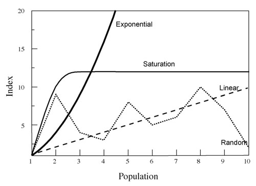
Figure 1. Some relationships that can occur between an index of population size and actual population size. Although many relationships are possible as illustrated (including no real relationship), most indices assume a linear relationship, usually a 1:1 linear relationship in which any proportional change in the index reflects the exact same proportional change in the population.

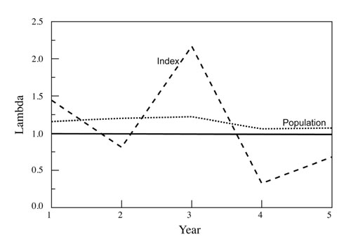
Figure 2. The finite rate of population increase (lambda) as predicted by an index of population change (in this case a CPUE index, the number of ibex observed per camera-day) and actually observed for the population over a 5-year period. The x-axis is the finite rate of population increase, or lambda, which is simply the increase in population size relative to 1.0 (>1 = a growing population, <1 = a declining population); a value of 1.0 represents no change (the solid black line). In this case, the actual population increased each year by 6–22% (i.e., lambda = 1.06–1.22), whereas the index indicated increases in some years and declines in others, and included annual magnitudes of change (i.e., lambda = 2.17 from Year 2 to Year 3, which would be more than a doubling in population size) that were well outside the biological potential of ibex.

Trend indices also require that a large, geographically distributed sample of the population is surveyed so that the index can be reasonably reflective of the population as a whole. Consequently, sampling must be fairly intensive and cover a significant portion of the area or ranch. Most commonly, private managers conduct only one or two spotlight surveys across a limited portion of their ownership based on the recommendations of consultants, and these surveys are seldom replicated. Almost never is the actual power of the index to detect a change considered when a survey strategy is set up on private lands. Rather, trend index surveys are frequently established for ease of data collection, under the impression that the data is valid. The usual result of this is that the sampling intensity is far too low to actually detect any annual or multi-annual trends because of high variability among survey transects or replicates (Figure 3). The more variable surveys are, the greater the number of replicates needed to actually detect a change. Seldom will even three replicates be sufficient to detect a true change in a population, and two replicates or a single unreplicated survey cannot reliably give actual trend information unless it covers the entire ranch and is corrected for missed individuals (and at which point it becomes a population estimator, not a trend index; see Bender, 2020).

Figure 3. Spreadsheet illustrating numbers of deer counted over 10 transects (this could be thought of as numbers counted per camera for 10 camera traps, numbers seen per survey for 10 spotlight surveys, numbers seen over 10 replications of a single ground survey, numbers of pellet-groups counted per transect for 10 transects, etc.). Note that both Example 1 and Example 2 indicate that the population increased based on average observations of 6.9 deer per transect (or replicate) in Year 1 and 9.6 deer observed/transect (or replicate) in Year 2. However, when the variability of the results (i.e., the differences in counts among transects/replicates) is analyzed and used to create 90% confidence intervals (CIs), only in Example 2 did deer actually show a statistically significant increase (as shown by 90% CIs that DO NOT overlap). In Example 1, the overlapping CIs between the Year 1 and Year 2 indices indicate no actual detectable difference. Why? Because the variability of the data, whether expressed as the sample variance, standard error (SE), or width of the 90% CIs, is much greater in Example 1 for each year. Equations used to determine the confidence intervals in Excel are shown in the middle box referenced to the Example 1 Year 1 data (i.e., column B in the spreadsheet).

Because of these issues, most applications of trend indices provide little or no reliable information for managers. Remember, in order for a trend index to have any real relationship to abundance, the methodology must be consistent, sampling must be representative and intensive enough to reliably describe the population, and the relationship between the index and population trend must not be influenced by any environmental variation that is uncontrolled (or these factors must be included as covariates in trend analyses). These constraints, especially the latter, are seldom considered with most applications of trend indices.

Environmental variation in particular can cause the assumption of a homogenous and proportional relationship between abundance and the index to be violated, and thus needs to be addressed in sampling strategies. Sampling strategies, such as stratified-random (as opposed to purely random) strategies, attempt to account for vegetation type or other fairly constant environmental attributes that vary among survey areas or times. By stratifying surveys according to environmental differences, the overall index may better represent the actual population trend (Härkönen and Heikkilä, 1999; Keegan et al., 2012). This type of stratification is commonly done when surveys are associated with roads or trails because these are not randomly located across the landscape and the actual area sampled is often very small (i.e., the sample is poorly distributed, being associated with only a narrow band along the road or trail). However, a big potential negative effect of stratified-random or systematic sampling is that you may not capture all of the environmental variation across the landscape due to your sampling not being random. This problem is often addressed by ensuring that stratification (blocking) includes all relevant variables in the stratified effect (for example, all the habitat types present on a ranch, etc.). A related problem is that many significant environmental influences cannot be predicted a priori, such as precipitation. They can only be included in a posteriori analyses, and this is almost never done by managers.

Another attempt to deal with environmental variables that may affect the relationship between abundance and the index includes standardization of survey methodology, which is most often used to account for seasonal and observer effects. However, many—probably most—important environmental factors can only be included and accounted for in models that relate abundance and the index after the fact, i.e., in multi-annual analyses; this negates the primary purpose of why many managers use trend indices, which is to detect annual changes in relative abundance.

Despite these limitations, if managers do desire to obtain reliable trend information, the following sections describe the most commonly used trend indices for wildlife enterprises and provide information on their application and the sampling intensity needed to overcome some of the issues noted above. Managers should remember that these are very general guidelines, and surveys should be designed specifically for the local attributes of wildlife enterprises. Additionally, the actual intensity of sampling needed for detection of trends should be determined from the variation among the surveys on each property (i.e., the dispersion among statistical replicates).

Catch-Per-Unit-Effort (CPUE)

CPUE indices are currently mostly associated with the use of intensive camera trapping surveys (Figure 4). CPUE indices scale “catch” by an estimate of “effort”; in the case of camera trapping surveys, this is usually numbers of individual animals of the target species photographed divided by the total number of days cameras have been deployed and were functional (i.e., individuals/camera-day). While CPUE surveys are relatively inexpensive, are easy to collect, and have a strong empirical background in fisheries management, they are strongly influenced by changes in vulnerability of individuals to capture (e.g., weather conditions, etc.) as illustrated above (Figure 2). Because of complications with replication of surveys, they are most often used in multi-annual analyses employing regression techniques, with the index modeled as a function of year. (In this Circular, I will only describe statistics for simple year-to-year comparisons. If more advanced techniques are desired, such as multiyear regression modeling, managers should contact CES Agents or Specialists directly [https://aces.nmsu.edu/county/)].)

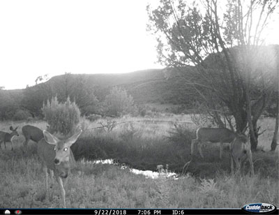
Figure 4. Camera traps can allow monitoring of populations 24/7/365. Properly designed camera trap surveys can provide information for catch-per-unit-effort trend indices and sex and age ratios, and allow individual identification of certain components of the population, including bucks and bulls. (Photo courtesy of L. Bender.)

CPUE indices assume that catch is proportional to the size of the population, and that it varies only with population size. As noted above, both of these assumptions are probably wrong in most cases, but the latter can potentially be corrected for if the variables thought to influence catch (other than abundance) are known and sample size is large. For example, if cameras are placed at permanent water sites, then CPUE may simply reflect differing proportions of individuals that use these sites as precipitation (and hence other ephemeral water sources and forage moisture content) varies. Thus, the numbers of photographic captures may simply reflect variable use of water sites annually, rather than any change in population size. This problem can be addressed by camera placement, i.e., developing an extensive camera-trapping grid that is placed randomly (or stratified randomly) across the area/ranch in order to provide greater distribution of the sample and make more of the population vulnerable to photographic capture (not just those in close proximity to permanent water).

Independence of photographic capture is another issue. Most surveys use a camera delay of 5 minutes between photographic captures, but individuals may remain at the camera site far longer than that, especially around water sources. Consequently, the same individuals may be photographed several times in a short period; for example, perhaps five photos of the same group in a 20-minute period. In these cases, independence of capture can be addressed by using only the highest count from this group of pictures, rather than totaling all individuals in each of the five pictures. This problem is exacerbated by camera delays of <5 minutes, and for “burst” settings that shoot multiple pictures in a few seconds.

Additionally, comparisons among differing management units that vary significantly in habitat are a problem because CPUE reflects both abundance and vulnerability to capture, and vulnerability can change significantly with the amount of security cover.

Application

1. Develop a camera grid that covers as much of the area as possible (i.e., cover the full extent of the study area or ranch if possible). Ideally, a grid will be placed so that every individual is vulnerable to capture. For example, if mule deer (Odocoileus hemionus) females have a home range of 2–3 mi2, then a grid with spacing of one camera per two sections would be ideal for mule deer. Since the number of cameras needed to cover large ranches would be extremely large, a spacing of 2–5 mi is often used for very large ownerships (i.e., >100 sections).
   
   
2. In the near vicinity of each randomly (or stratified-random) selected site, place cameras where individuals are likely to be captured, such as along a trail or the edge between adjacent habitat types near the random point. Cameras are best positioned so that they shoot to the approximate north (to avoid the glare of the sun) and programmed for a 5-minute delay between photographs (to limit non-independent photographs).
   
   
3. Run cameras all year or at least seasonally; if seasonally, keep the time of use consistent among years.
4. Pay attention to the number of days cameras are functional to accurately track camera-days. If a camera is knocked down or otherwise not functional for 30 d in a 90-d period, then the number of camera-days equals 60, not 90. Nonfunctional cameras can usually be detected by an abrupt end of photos after a certain date, and the time a camera was knocked down is easily determined because it is usually photographed and the aspect changes (e.g., starts shooting the sky or ground).
   
   
5. The index is numbers of individuals photographed per camera-day. For example, if each of 20 cameras is treated as an independent replicate and each camera averaged 100 individual deer photographed over 50 camera-days, then CPUE = 2.0 deer/camera-day with a confidence interval (CI) of +0 deer/camera-day. In other words, the average or mean number of deer photographed per camera-day is 2.0, and because each of the cameras was exactly the same (all averaged 2.0 deer/camera-day), there is no variation among the cameras, and thus the range of the CI = 2.0–2.0. However, independent replicates virtually never give the same exact data, so there will be variation among the replicates (Figure 3). The amount of that variation determines how wide CIs are and whether they overlap or not; in other words, whether the index actually differs between sampled periods or years (Figure 3). Figure 3 illustrates how the exact same change in an index may or may not actually differ statistically depending on how much variation there is in the survey results.
   
   
6. If all cameras are pooled for a multi-annual analysis, the calculation incorporates all cameras in the survey grid. For example, if 700 individual deer are photographed among 20 camera sites that were operational for 50 days each, then CPUE = 0.7 deer/camera-day.
   
   
7. Replication can be an issue with CPUE camera surveys. If each camera is (properly) treated as an individual replicate, the variation in photographic captures among cameras is frequently extremely large (for example, a camera near a permanent water site may have thousands of pictures per month, whereas a camera in dense pinyon-juniper woodland may have <10). The resulting variation makes detection of annual changes extremely difficult. Because of this, sites at strong attractants (i.e., water, feeding stations, etc.) are often not included in the trend grid, and are used for other purposes such as individual identification (see below). Even then variance can be large, so CPUE data is most often used in multiannual regression analyses with data from all cameras pooled into a combined photographs/camera-day, as above. The problem here is that without an estimate of variance for the sample, comparisons between years cannot be statistically tested.
   
   
8. Managers can extrapolate CPUE to estimate population abundance using DeLury non-linear harvest-per-unit-effort or similar models if advanced applications are desired (Roseberry and Woolf, 1991; Skalski et al., 2005).

Individual Identification

Photographic captures from camera-traps may allow individual identification of some members of the population, such as mule deer bucks or elk (Cervus elaphus) bulls (Figure 5). Some highly experienced observers can identify individual males by antler characteristics within a year, and this can be used as a minimum count (or minimum population estimate) for that population component (Jacobson et al., 1997; Beaver et al., 2016). If unbiased herd composition data (i.e., male:female and juvenile:female ratios) is available, this minimum can be extrapolated to a minimum estimate of the entire population (Bender and Spencer, 1999; Bender, 2006, 2019; Beaver et al., 2016). This method has been primarily used in the southeastern United States with white-tailed deer (O. virginianus), on much smaller ownerships with much higher deer densities than seen in New Mexico and elsewhere in the West. Whether it can be useful under conditions typical of New Mexico is unclear. Consequently, I have been testing this approach on a ranch in northern New Mexico with mule deer. In this study, at least two highly experienced people independently go through all photographs from the autumn season and attempt to determine the minimum number of males that they are certain are different individuals. This information is being compared with other data (i.e., sightability population estimates [Bender, 2012], photographic capture rate) and initially appears to be reflective of the actual abundance of bucks. Moreover, very advanced camera-based survey methods involving individual identification, such as Time-in-Front-of-Camera approaches (Huggard, 2018; Warbington, 2020), continue to be developed. These advanced methods can produce rigorous population or density estimates in addition to trend information. While these approaches are not detailed here, very advanced users of camera-based surveys may want to investigate these newer, more intensive, and more advanced uses of individual identification approaches.

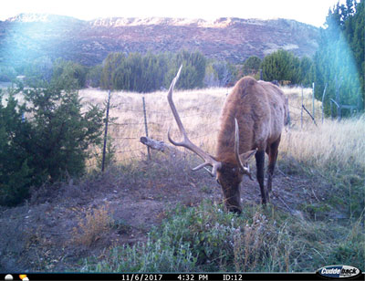
Figure 5. Camera trap data can allow identification of unique individuals in the population, which can aid in determining trends. Identification of individuals can occasionally be obvious, as with this bull elk, but is usually much more difficult and requires more than one highly experienced observer for corroboration of individuals. (Photo courtesy of L. Bender.)

Application

1. Have two or more experienced observers independently go through all photographs of males taken during the late summer–autumn period (around August–December).
   
   
2. Identify the minimum number of males that observers are sure are unique individuals based on antler characteristics. If not 100% certain, then do not count that individual as unique from the other known individuals.
   
   
3. Camera-trapping grids should be set up to cover the area adequately as described in CPUE above for maximum benefit. Because this method is attempting to identify only distinct individuals and not population trend per se, less intensive camera trapping grids can be used (i.e., such as placing cameras at water sites only).
   
   
4. The index is simply the number of known individuals annually. The change in this minimum number of known individuals can be the trend (for that population component only) if sampling is identical each year (i.e., as long as camera placement and timing are consistent among years).

Minimum Counts

A minimum count represents the absolute minimum number of individuals known to be present in a given area, such as a ranch. In this sense, it is similar to the individual identification index discussed above, but does not require identifying individual animals. With this method, an attempt is made to census the entire population (i.e., enumerate or count all individuals present in the area). In reality, an unknown proportion of the population is seen and counted, but no attempt is made to determine what that proportion is or to correct the count for it, as with sightability models or other population estimators (Keegan et al., 2012; Bender, 2020). Most frequently, minimum counts are done using helicopter or fixed-wing aerial surveys flown over the entire evaluation area (or a significant portion of it); however, some other techniques (e.g., ground counts, spotlight counts, etc.) can also yield much lower minimum counts. The difference is that true minimum counts usually attempt to cover the entire area and census the population, whereas spotlight and similar ground counts are assessing only a much smaller portion of the population (Figure 6).

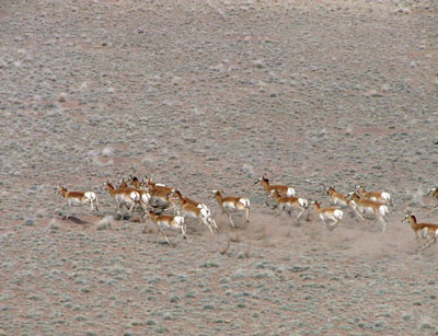
Figure 6. Minimum counts from either helicopter or fixed-wing surveys allow coverage of much greater areas than do ground or spotlight counts. Because of this, they are much more likely to reflect the actual population, as well as result in less biased composition data if conducted during appropriate periods. (Photo courtesy of E. Watters.)

This method provides managers with an absolute minimum number of individuals present, which is often better accepted by many people than are sample-based population estimates because sampling techniques, statistical inference, and probability are often poorly understood (Keegan et al., 2012). Helicopter counts provide more accurate sex and age classification than do ground-based and fixed-wing counts because of longer observation times, closer proximity to animals, ability to herd animals to provide optimal viewing opportunities, and ability to observe animals in inaccessible areas (Bender et al., 2003). Generally, if applied using helicopters, managers are much better off incorporating sight-bias flight protocols (Bender, 2020) to derive an actual population estimate, rather than a minimum count.

More so than other methods, techniques to collect minimum count data are rapidly evolving. For example, drones are being increasingly used to conduct minimum counts (Linchant et al., 2015) using both high-resolution cameras and forward-looking infrared (FLIR) cameras, often both together because FLIR is superior at detecting the presence of animals, whereas high-resolution photographs are superior in identifying the species detected. This method is applicable to fixed-wing flights as well, which cost substantially less (<1/5) than the cost of helicopter surveys. For example, counts using synchronized FLIR and high-resolution cameras have been used to count multiple species (Millette et al., 2011). While this technology is still in development, its future use has the potential to allow essentially total counts of larger species at the cost of fixed-wing flights. While current-generation drones may be useful for very small ownerships or aggregated individuals (such as elk at feeding stations), large ownerships still require manned aircraft barring significant advances in non-military technology.

Application

1. Minimum counts are usually conducted from either helicopters or fixed-wing aircraft, with flight protocols (such as airspeed, altitude above ground level, and spacing of transect lines) and observer behavior (including number of observers, direction of observation, and width of transect lines) held constant among surveys (see Bender, 2020, for an example of appropriate flight protocols). In some cases, experimental techniques, such as the use of aerial photographs to obtain counts of concentrated individuals or thermal imaging, have been used (Russell et al., 1996; Lancia et al., 2005).
   
   
2. Aerial surveys are flown with consistent flight protocols to ensure consistent and near total coverage of sampled areas, and are converted to individuals observed/unit area or individuals observed/hour to obtain the population index. Aerial counts for population trend, as contrasted with counts used solely for sex and age composition, usually have much more specific survey protocols that are similar to those required for abundance estimators, such as sightability models (see Bender, 2020). Despite this, like sightability models and similar methods, estimates will always be negatively biased because topography and other visual barriers will prevent complete observation of survey units.
   
   
3. The index is the number of individuals counted if the same area(s) are counted each year, or the number of individuals/hour if sampled areas vary among years. Usually, the entire area is surveyed annually (or the same areas are surveyed annually).
   
   
4. Variations of minimum aerial counts are the most commonly used trend indices for big game, and these minimum counts are frequently converted to estimates of population abundance, often by correcting counts for different likelihoods of observing individual animals based on habitat types or other environmental influences (Bender, 2020), stratifying surveys based on habitat type (Bartmann et al., 1986; Freddy et al., 2005), or by assuming all individuals along the aerial transect were seen and estimating the width of the transect using distance sampling methods to correct for varying detection probabilities based on habitat type, transect width, or other variables (Thomas et al., 2010).

Spotlight Surveys and Ground Counts

Spotlight surveys and ground counts are similar, with spotlight surveys differing by being conducted at night when big game may be less hesitant about using open habitats or areas adjacent to roads. Both spotlight surveys and ground counts are used to collect minimum count and herd composition data (Figure 7). Routes need to be standardized, replicated, and driven at the same time each year. Standardization of surveys is necessary because detection probabilities can vary with habitat conditions, weather, disturbance, etc.

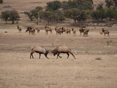
Figure 7. Ground or spotlight surveys can also collect minimum count data for trends, but must be carefully designed and replicated because usually only a very limited portion of ranches is actually surveyed (i.e., only a narrow band along roads). (Photo courtesy of M. Rearden.)

If conducting spotlight surveys, it is a good idea to contact your local agency Game Warden and let them know you will be conducting spotlight counts. Spotlight counts can generate concern among adjacent residents and reports of illegal hunting. To emphasize, spotlight or ground surveys must be replicated and routes must cover a substantial proportion of the area/ranch (see below) to try to sample a representative proportion of the population (a more rigorous sampling strategy is needed because numbers actually seen will be much lower than numbers seen in aerial minimum counts, above). A single survey of a limited area provides NO insight into population trend, despite being the most commonly recommended (and used) index on private ranches in New Mexico.

Application

1. Ground counts are best conducted from vehicles, but occasionally may be done from horseback or by hiking.
   
   
2. Transects should be distributed throughout the area, allow coverage of as much of the area as possible, and be representative of the various habitat types present in the area.
3. As a general rule, total transect length (in miles) should equal >50% of the area/ranch size (in sections) for smaller ranches (<100 sections; the smaller the ranch, the higher the proportion) and >25% for larger ranches. For example, if a ranch = 100 sections, there should be a minimum total of about 50 mi of transects. For a 10-section ranch, transects should total at least 10 mi and preferably more.
   
   
4. Transects are usually about 10–20 mi long so that they can be driven at approximately 5–10 mph in the 2 hours prior to dark or the first 2 hours in the morning. The necessary total length of transects can be split among several shorter transects to get better spatial coverage of the area. For example, if 100 mi of transect are necessary, this can be accomplished with five 20-mi transects.
   
   
5. Surveys are usually driven during the early morning or late evening when big game activity is highest for the diurnal period. Spotlight surveys are conducted shortly after dark when animals are more active and may be less hesitant about using areas closer to roads. Sampling protocols are identical for both spotlight and ground surveys.
   
   
6. To conduct surveys, a driver navigates a vehicle along a permanently established route, while an observer (or two) records all big game animals seen and preferably classifies individuals by sex and age class for composition data (see Bender, 2006, 2019). The method is similar with spotlight surveys, with the addition that the observer(s) shine a spotlight along the side of the route to detect individuals, while determining composition may not be possible.
   
   
7. The survey should be saturated with observer teams if more than one transect exists. For example, if survey routes cover an area that would take four surveys to cover by one team, use four teams to finish in one evening/morning to completely survey the area in one time period. Surveys should be replicated at least three times, with either the highest total count or the average numbers of animals or animals/mile used as the trend index.
   
   
8. Typically, total numbers counted or number of animals seen/mile of route serves as an index to annual changes in abundance, and sex and age composition provides trend information on population demographics (Bender, 2019). Surveys can be compared between years by calculating confidence intervals around the mean count (or mean number per mile) based on the replicates and seeing if the confidence intervals overlap (Figure 8).
   
   
9. Surveys should be performed at the same time each year when the local population is likely to consist solely of resident animals. For example, do not survey during winter if on winter range after migration of other individuals into the local population (unless you are interested in the wintering population rather than the local resident population).
   
   
10. Distance sampling methods, including stratification by habitat types, animal behavior, etc., can be used to extrapolate minimum counts to abundance estimates (Thomas et al., 2010).

Figure 8. Example showing analysis of a long spotlight or ground count survey that was split into three segments (segments 1a, 1b, and 1c) to allow completion of the transect in one evening, and that was replicated three times. As in Figure 3, the averages from the three replicates are the same in both examples, but only Example 2 shows an actual detectable statistical difference between Year 1 and Year 2. The much greater variation among the three survey replicates in Example 1—particularly in Year 1—results in much wider CIs (i.e., ±6.9 as opposed to ±2.0 in Example 2). This results in overlapping CIs between Years 1 and 2 in Example 1, and thus no real detectable increase from Year 1 to Year 2 in Example 1. Equations used to determine the confidence intervals in Excel are shown in the middle box referenced to the Example 1 Year 1 data (i.e., column B in the spreadsheet).

Pellet-group Counts

Pellet-group surveys are a commonly used index, especially for relative use of habitats, but occasionally for population trend as well (Neff, 1968). The index involves counting the number of pellet-groups of the target species found in plots or belt transects, and the average number of groups among plots/transects is then used as a trend index. Pellet-group counts for population trend are most frequently conducted on seasonal ranges, such as winter range. Because habitats are not uniform and pellet-group distribution depends on relative habitat use, pellet-group transects are often stratified among vegetation types (Neff, 1968; Härkönen and Heikkilä, 1999). For accuracy, permanent transects that are cleared of old pellet-groups after each survey should be used to eliminate confusion in aging pellet-groups.

Pellet-group counts are relatively easy to conduct and have been correlated with other trend indices, including aerial minimum counts and hunter observations (Härkönen and Heikkilä, 1999), suggesting that they can be a reliable index under certain conditions. However, there are a number of factors that can affect the results of pellet-group transects. First, it can be difficult to distinguish pellet-groups by species if several species of ungulates are present. Additionally, size and shape of plots (e.g., belt transects vs. circular plots) and sampling effort strongly affect results (Härkönen and Heikkilä, 1999). Strict criteria need to be established and followed as to what constitutes whether a group is considered in or out of the plot/transect. For example, a manager may decide that if any pellets of a group are within the plot/transect, then the group should be counted. Another may exclude any group that is not completely within the plot/transect. Either criterion is correct as long as it is applied consistently. Even with rigorous standardization of these and other potential sources of bias, the power of pellet-group transects to detect trends frequently is low, particularly for low-density populations.

Application

1. This method involves clearing permanent plots or belt transects of accumulated pellet-groups and returning after a specified time period (usually one year) to count the number of new pellet-groups. Plots or transects should be counted after an identical length of time following clearing. Most commonly, transects are cleared while counting, then revisited after one year and counted and cleared again.
   
   
2. Randomly (or stratified-random) place 100-m (or yard) transects and count all pellet-groups within 1 m (or yard) of each side of the line for a 100 × 2 m (or yard) belt transect. A reasonable sample size would be one per section for small (<50 sections) areas/ranches, and one per two sections for larger areas/ranches. Transects should be distributed throughout the property. If vegetation monitoring transects are done on a ranch, pellet-group transects can be placed along the same transect and conducted simultaneously to save time and effort.
   
   
3. The average number of pellet-groups among transects serves as the index to abundance. As discussed under CPUE indices above, variation among transects can be large, especially if some are at or near attractants, such as permanent water or feed stations. Because of this potentially significant variation among transects, annual changes often need to be large to detect actual differences. Annual counts can be compared using confidence intervals based on the variation among transects (Figure 3).
   
   
4. Although used as a trend index or abundance estimator, pellet-group counts are usually more valuable in determining relative habitat use patterns (Neff, 1968; Härkönen and Heikkilä, 1999).
   
   
5. Extrapolation to population abundance requires further assumptions, including 1) constant defecation rates, 2) exact knowledge of time of use in days, and 3) population density is uniform throughout range. For abundance estimation, there is little validation of most commonly used daily defecation rates, which undoubtedly vary with season, diet, etc. Despite this, pellet-group indices are occasionally converted to densities by dividing by the “guesstimated” number of times an animal defecates/day and the number of days plots were exposed. For example, if you assume that a deer defecates 10 times/day and after 10 days you find 700 pellet-groups/acre, it is assumed that 7 deer were present (7 deer × 10 days × 10 pellet-groups/day/deer) (Neff, 1968; Härkönen and Heikkilä, 1999).

Acknowledgments

I thank C. Allison, New Mexico State University; R. Baldwin, University of California–Davis; A. Darrow, Canon Bonito Ranch; and T. Kavalok, Alaska Department of Fish and Game, for insightful critiques of this Circular, and members of the WAFWA Mule Deer Working Group for many discussions on this subject.

Literature Cited

Bartmann, R.M., L.H. Carpenter, R.A. Garrott, and D.C. Bowden. 1986. Accuracy of helicopter counts of mule deer in pinyon-juniper woodland. Wildlife Society Bulletin, 14, 356–363.

Beaver, J.T., C.A. Harper, L.L. Muller, P.S. Basinger, M.J. Goode, and F.T. Van Manen. 2016. Current and spatially explicit capture-recapture analysis methods for infrared triggered camera density estimation of white-tailed deer. Journal of the Southeastern Association of Fish and Wildlife Agencies, 3, 195–202

Bender, L.C. 2006. Uses of herd composition ratios in ungulate management. Wildlife Society Bulletin, 34, 1225–1230.

Bender, L.C. 2019. Using population ratios for managing big game [Circular 669]. Las Cruces: New Mexico State University Cooperative Extension Service.

Bender, L.C. 2020. Guidelines for monitoring big game numbers in New Mexico I: Population estimation [Circular 664]. Las Cruces: New Mexico State University Cooperative Extension Service.

Bender, L.C., and R.D. Spencer. 1999. Estimating elk population size by reconstruction from harvest data and herd ratios. Wildlife Society Bulletin, 27, 636–645.

Bender, L.C., W.L. Myers, and W.R. Gould. 2003. Comparison of helicopter and ground surveys for North American elk Cervus elaphus and mule deer Odocoileus hemionus population composition. Wildlife Biology, 9, 199–205.

Davis, D.E., and R.L. Winstead. 1980. Estimating the numbers of wildlife populations. In S.D. Schemnitz (Ed.), Wildlife management techniques manual, fourth ed. (rev.) (pp. 221–245). Washington, D.C.: The Wildlife Society.

Freddy, D.J., G.C. White, M.C. Kneeland, R.H. Kahn, J.W. Unsworth, W.J. deVergie, V.K. Graham, J.H. Ellenberger, and C.H. Wagner. 2004. How many mule deer are there? Challenges of credibility in Colorado. Wildlife Society Bulletin, 32, 916–927.

Fuller, T.K. 1991. Do pellet counts index white-tailed deer numbers and population change? Journal of Wildlife Management, 55, 393–396.

Härkönen, S., and R. Heikkilä. 1999. Use of pellet group counts in determining density and habitat use of moose Alces alces in Finland. Wildlife Biology, 5, 233–239.

Huggar, D. 2018. Animal density from camera data. Edmonton, Alberta: Alberta Biodiversity Monitoring Institute.

Jacobson, H.A., J.C. Kroll, R.W. Browning, B.H. Koerth, and M.H. Conway. 1997. Infrared-triggered cameras for censusing white-tailed deer. Wildlife Society Bulletin, 25, 547–56.

Keegan, T.W., B.B. Ackerman, A.N. Aoude, L.C. Bender, T. Boudreau, L.H. Carpenter, B.B. Compton, M. Elmer, J.R. Heffelfinger, D.W. Lutz, B.D. Trindle, B.F. Wakeling, and B.E. Watkins. 2012. Guidelines for monitoring mule deer populations. Tucson, AZ: Mule Deer Working Group, Western Association of Fish and Wildlife Agencies.

Kufeld, R.C., J.H. Olterman, and D.C. Bowden. 1980. A helicopter quadrat census for mule deer on Uncompahgre Plateau, Colorado. Journal of Wildlife Management, 44, 632–639.

Lancia, R.A., W.L. Kendall, K.H. Pollock, and J.D. Nicholls. 2005. Estimating the number of animals in wildlife populations. In C.E. Braun (Ed.), Techniques for wildlife investigation and management (pp. 106–153). Bethesda, MD: The Wildlife Society.

Linchant, J., J. Lisein, J. Semeki, P. Lejeune, and C. Vermeulen. 2015. Are unmanned aircraft systems (UASs) the future of wildlife monitoring? A review of accomplishments and challenges. Mammal Review, 45, 239–252.

Millette, T.L., D. Slaymaker, E. Marcano, C. Alexander, and L. Richardson. 2011. AIMS-Thermal—A thermal and high resolution color camera system integrated with GIS for aerial moose and deer census in northeastern Vermont. Alces, 47, 27–37.

Neff, D.J. 1968. The pellet-group count technique for big game trend, census, and distribution: A review. Journal of Wildlife Management, 32, 597–614.

Russell, J., S. Couturier, L. Sopuck, and K. Ovaska. 1996. Post-calving photo-census of the Rivière George caribou herd in July 1993. Rangifer, 16, 319–330.

Skalski, J.R., K.E. Ryding, and J.J. Millspaugh. 2005. Wildlife demography. Burlington, MA: Elsevier.

Thomas, L., S.T. Buckland, E.A. Rexstad, J.L. Laake, S. Strindberg, S.L. Hedley, J.R.B. Bishop, T.A. Marques, and K.P. Burnham. 2010. Distance software: Design and analysis of distance sampling surveys for estimating population size. Journal of Applied Ecology, 47, 5–14.

Warbington, C.H. 2020. Sitatunga population ecology and habitat use in central Uganda [Dissertation]. Edmonton: University of Alberta.

Williams, B.K., J.D. Nichols, and M.J. Conroy. 2001. Analysis and management of animal populations. San Diego, CA: Academic Press.

For further reading

CR-662: Guidelines for Management of Habitat for Mule Deer: Piñon-juniper, Chihuahuan desert, arid grasslands, and associated arid habitat types
https://pubs.nmsu.edu/_circulars/CR662/

CR-664: Guidelines for Monitoring Big Game Populations in New Mexico I: Population Estimation
https://pubs.nmsu.edu/_circulars/CR664/

CR-669: Using Population Ratios for Managing Big Game
https://pubs.nmsu.edu/_circulars/CR669/

Lou Bender is a Senior Research Scientist (Natural Resources) with the Department of Extension Animal Sciences and Natural Resources at NMSU. He earned his Ph.D. from Michigan State University. His research and management programs emphasize ungulate and carnivore management, integrated wildlife and livestock habitat management, and wildlife enterprises in the Southwest and internationally.

To find more resources for your business, home, or family, visit the College of Agricultural, Consumer and Environmental Sciences on the World Wide Web at pubs.nmsu.edu.

Contents of publications may be freely reproduced, with an appropriate citation, for educational purposes. All other rights reserved. For permission to use publications for other purposes, contact pubs@nmsu.edu or the authors listed on the publication.

New Mexico State University is an equal opportunity/affirmative action employer and educator. NMSU and the U.S. Department of Agriculture cooperating.

November 2021 Las Cruces, NM