Circular 651

Revised by J. Michael Patrick and Don P. Blayney

College of Agricultural, Consumer and Environmental Sciences, New Mexico State University

Respectively, Associate Professor and Research Assistant Professor, Department of Agricultural Economics and Agricultural Business, New Mexico State University. (Print Friendly PDF)

Introduction

Between 2010 and 2018, the state of New Mexico experienced population growth and an expanding economy, but rural areas lagged behind urban areas. Key economic and demographic factors shaping rural life in New Mexico examined here include population, migration, employment, unemployment, farm income, poverty, and education.³ Knowledge of trends in these factors and their causes can inform the actions of local officials and policy makers focusing on efforts to address economic development challenges facing rural New Mexico communities.

Population Change in Rural New Mexico, 2010–2018

Various economic studies suggest that population (or population growth) and economic performance are positively correlated in particular localities. However, defining a causal relationship between the two variables often is a “chicken or egg” issue. It is certainly plausible that localities with higher economic growth may attract more people. It is also conceivable that localities faced with high poverty may experience population declines as residents leave due to a lack of employment opportunities.

According to the U.S. Census Bureau, the total state population was about 2.1 million people in 2018. Figure 1 shows a steady state-level population growth between 1969 and 2008 that continued after 2008, but at a slower rate. The year 2008 is an important benchmark in economic studies because it is commonly associated with the beginning of the “Great Recession,” which lasted until early in 2010.

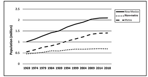
Figure 1. State of New Mexico, metro, and non-metro area populations, 1969–2018.

Between 2010 and 2018, the U.S. population growth rate was about 5.8%, while it was only about 1.5% in New Mexico. The small positive state population growth is a result of a substantial difference between the rural (non-metro) and the urban (metro) areas in New Mexico. Not only has rural county growth generally lagged behind their urban counterparts, the gap widened from 1969 to 2008 before leveling off somewhat.

Twenty rural counties had negative population growth from 2010 to 2018. Hidalgo county reported the highest population loss during this period (-14.7%), followed by De Baca (-13.9%), Colfax (-13.4%), Union (-10.3%), and Quay (-9.9%). Six rural counties showed positive population growth between 2010 and 2018: Lea (7.2%), Eddy (6.9%), Los Alamos (5.5%), Otero (3.6%), Curry (1.0%), and McKinley (0.9%). Among urban counties, the fastest-growing county in the state, Sandoval, grew by 8.8% over the 2010–2018 period, followed by Santa Fe (3.7%), Doña Ana (3.4%), and Bernalillo (2.2%). The three other urban counties lost population: Torrance the most (-5.2%), followed by San Juan (-4.1%) and Valencia (-0.4%) (see Table 4).

Given the relative stability of current birth and death rates, a critical demographic factor for assessing population growth or decline in a locality is the mobility of people, commonly shown by net migration levels. Between 2010 and 2017, the net migration for New Mexico was about -2.8%. Both rural and urban areas had negative net migration: 22 of 26 rural counties and 5 of 7 urban ones. Four rural counties—Eddy, Los Alamos, Harding, and Sierra—had positive net migration rates less than 3%. The highest net out-migration rates in the rural counties were in Hidalgo, Roosevelt, and Colfax counties. The two positive net migration urban counties were Sandoval (7.1%) and Santa Fe (2.7%), while San Juan (at almost -11%) posted the highest out-migration rate of all the urban counties (see Table 4, Figure 2).

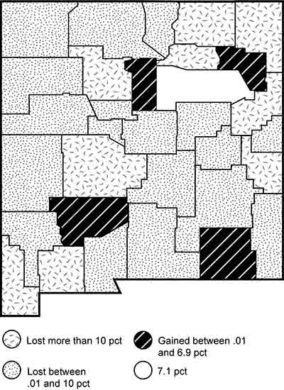
Figure 2. Population net migration of New Mexico counties, 2010–2017.

Identifying the underlying reasons for out-migration requires in-depth analyses. Those analyses might focus on the loss of earning opportunities in agriculture, declining farm support programs, differences between urban and rural wages, existing levels of unemployment in rural areas or better employment opportunities in urban areas, relocation of manufacturing plants in urban and/or suburban areas, and lack of either (or both) social and natural amenities.

Government officials, business leaders, and economic development practitioners need to understand factors associated with population changes. Population declines can impose higher costs on those who remain in order to keep public services operating. If the higher costs are too high, a further population exodus can threaten the existence of rural communities. A second factor that has significant implications for many rural areas is the changing role of agriculture. Farm and ranch operations have been instrumental in sustaining rural economies, but as their number has declined, the availability of off-farm employment opportunities, including non-farm self-employment, has become more important in rural economies.

Employment

Employment growth is closely associated with population growth in a region. People often change places of residence based on both the availability of existing jobs and identified job market prospects in a locality. Population growth in a locality also creates new jobs because there will be an increase in demand for basic services, such as education, healthcare, roads, utilities, and retail businesses. Although employment in the non-metro areas in New Mexico has generally lagged behind their metro counterparts, the historical gap between the two appears to be narrowing.

Total employment in the state of New Mexico in 2010 was 1,059,977. Of that total, 728,466 were in urban areas (68.7%) and the remaining 331,531 (32.3%) were in the non-metro counties. In 2018, statewide employment had grown by almost 55,600 to 1,115,574. The metro and non-metro shares of the total were virtually unchanged at 769,770 (69%) and 345,804 (31%), respectively (Bureau of the Census, Bureau of Economic Analysis Regional Economic Accounts; http://www.bea.gov/regional/reis/). These aggregates do not show the underlying patterns of change that have occurred that are seen in Figure 3.

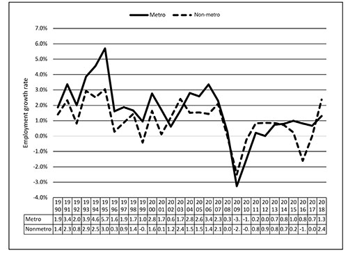
Figure 3. Employment growth rate in metro and non-metro areas in New Mexico, 1990–2018.

From Figure 4, we can see that some non-metro counties grew faster than other non-metro counties. Two rural counties—Colfax and Quay—had a negative employment growth during this time period.

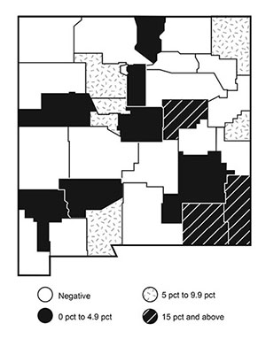
Figure 4. Total full- and part-time employment growth in New Mexico counties, 2010–2018.

Table 1 shows employment and employment changes between 2010 and 2017 for industry sectors for the non-metro areas of New Mexico. The industry sectors (NOT including the Other/Suppressed Industries category) are ordered by the number of persons employed in 2017. The top five employment sectors are Local Government (37,713), Transportation and Warehousing (34,666), Accommodation and Food Services (27,838), Construction (23,044), and Farm Employment (17,638). Only one of the top five sectors, Local Government, showed a decrease in employment over the period.

Specific employment changes in a selected local area are often assessed using shift-share analysis (SSA).⁴ SSA helps determine whether a particular local economy has experienced a faster or slower growth rate in employment than the larger economy. Compared with the larger economy, jobs in a local economy may be concentrated in some industries more than others based on the industrial structure of the local economy. For this reason, a locality with several fast-growing industries might display a high rate of employment gain. Similarly, a locality with several declining industries might experience a high rate of employment loss. More specifically, SSA allows us to analyze a change in the number of jobs in a locality in terms of structural changes, not just a general change in total employment in a locality.

SSA decomposes employment change in a region (over a given time period) into three contributing factors:

(1) The national growth effect represents the share of local employment growth that can be attributed to growth of the national economy. This component is based on the assumption that if the larger economy is experiencing employment growth, it is reasonable to expect that this growth will positively influence employment growth in a particular locality.

(2) The industrial mix effect represents the effects that specific industry trends at the national level have had on the change in employment in the locality. This component captures the fact that, at the national level, some industries grow faster or slower than others, and these differences are reflected in local industry structure. This component will highlight the industries in the locality that are increasing nationwide. A positive industry mix implies that the employment in the locality grew above the overall national average, and a negative industrial mix indicates the opposite.

(3) The competitive effect shows how industrial groups in the locality performed relative to those groups at national averages. A positive competitive share effect suggests that the locality increased its share of employment in that industry.

Table 2 presents the results of a shift–share analysis for rural New Mexico using an online calculation tool available at https://new-mexico.reaproject.org/analysis/shift-share/.

The positive national growth effect (44,543 jobs gained) offset the negative industry mix (6,221 jobs lost) and competitive share (30,700 jobs lost) effects to produce a net job gain of 7,622 for New Mexico rural counties between 2010 and 2017. The leading industries with net job gains were Construction (6,914), Accommodation and Food Services (3,153), Information (1,562), and Farm Employment (1,414). The industries with the highest net job losses were State Government (1,962), Federal Civilian (1,816), Local Government (1,574), and Retail Trade (894).

Unemployment

The overall economic performance in a locality is often linked to unemployment rates in the area. Historical data since 1990 for New Mexico show a steady decline in unemployment for both rural and metro counties until 2008 (Figure 5). With the onset of the Great Recession, unemployment in New Mexico’s metro and non-metro areas spiked to almost 9% before declining. Since 2008, the unemployment rates in the two areas have been at the same levels.

As Figure 5 indicates, there was a notable gap between the rates, with rural counties lagging behind their urban counterparts in this important economic indicator, but the gap narrowed. One potential reason for this narrowing may be out-migration of unemployed persons from rural counties. Both the rural and the urban unemployment rates were lower than the national average (4.6%) in 2007.

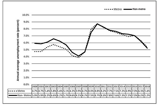
Figure 5. Trends in unemployment rate in metro and non-metro areas in New Mexico, 2000–2018.

Earnings

Figure 6 shows that average earnings per job in metro and non-metro areas began to diverge in the mid-1980s, and for the most part the gap widened until 2010. From about 1985 to 2000, the gap between rural and metro counties held steady, then narrowed in 2001, and again held steady for several years before narrowing in 2008. The onset of the Great Recession drove rural earnings down while having no noticeable effects on urban earnings, but they recovered to surpass urban earnings in 2011.

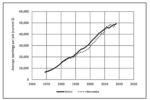
Figure 6. New Mexico metro and non-metro area average earnings per job, 1969–2018.

The patterns of metro and non-metro earnings are both more variable from 2008 to 2018, and since 2010, the patterns of both urban and rural earnings have become more variable compared to historical years. The average metro earnings per job rose from $44,655 in 2010 to $49,369 in 2018 (10.6%), while in the non-metro counties the average rose from $44,003 to $49,828 (13.2%). Both averages are below the U.S. average increase of 19.4% over the same period. Rural counties with the highest wage growth per job between 2010 and 2018 were Lee (55%), Eddy (49%), Cibola (43%), Harding (43%), and Hidalgo (41%).⁵

Farm Income Trends

The economic health of New Mexico’s production agriculture sector is closely linked to animal agriculture, primarily cattle and calves, as well as dairy (including milk products). Unadjusted gross farm income, direct government payments, and a set of other income sources comprise total farm income. As Figure 7 shows, trends in four agricultural income components in the state are quite different.

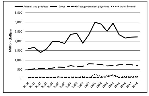
Figure 7. New Mexico gross farm income by source, 2000–2018.

Direct government payments and other income levels have been mostly flat and at low amounts. Crops income has been higher, but it also has shown only small changes over the period. There is a clear difference in animal and animal products over the period, with clear cycles in income appearing. The animal and animal products gross income rose significantly following the Great Recession to about $3 billion in 2011. Since that year, it fell (except for one rise in 2013) to about $2.1 billion in 2018. The volatility of gross farm incomes is mirrored by a similar situation with respect to the returns to farmers and ranchers in the state, as illustrated in Figure 8.

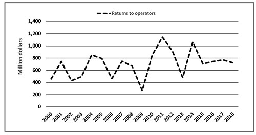
Figure 8. Returns to farm operators, 2000–2018.

As Figure 8 shows, there was a significant level of variability in returns to farm operators, but the long-term trend is upward. It is important for all to recognize, as farmers and ranchers do, that agricultural output prices can vary widely and at times rapidly.

Poverty

The overall individual poverty rate in New Mexico has averaged almost 19% from 1979 to 2018, peaking at almost 21% in 1989 (Table 3). The official poverty rate for the U.S. in 2018 was 11.8%.

Although relatively stable at the state level, individual counties exhibit a wide range of poverty. In 2018, 30 of New Mexico’s 33 counties (91%) had a poverty rate greater than 15% (Figure 9). If a benchmark poverty rate were set closer to the longer-term average based on Table 3—say 20%—the number of counties above that threshold is 21, or 70% of all counties.

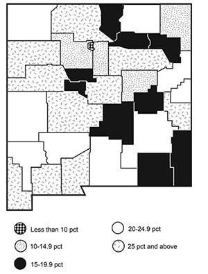
Figure 9. County-wide distribution of individual poverty rate in New Mexico, 2018.

These counties in general have had a poverty rate of 20% or more over the last three census periods. The national average for all non-metro counties in the U.S. has been fluctuating between 15 and 17% over the same time period.

Education

Educational attainment levels continue to improve in New Mexico. In 2016, the state high school graduation rate was about 71%. As has been the case historically, that rate was about 10% below the U.S. national level. There are several facets of education that are of interest in addition to overall graduation rates. Among them are the dropout rate, the high school or equivalent rate, or any one of several rates related to education beyond high school. Figure 10 shows a comparison between metro and non-metro areas of the state for selected educational attainment categories from 2010 to 2016.

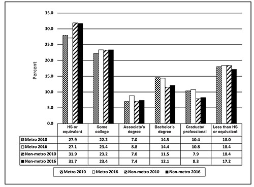
Figure 10. Educational attainment in New Mexico, 2010–2016.

Housing Stress Counties

Housing conditions often serve as a basis to classify localities such as states and counties. These conditions include the lack of complete plumbing, the lack of a complete kitchen, paying 30% or more of household income for housing costs, or having more than one person per room. Figure 11 highlights only one of these conditions: paying more than 30% of household income for housing costs. A significant result of this analysis is the clear difference between owner- and renter-occupied housing in the state.

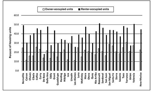
Figure 11. Housing units with costs 30% or more of household income, 2016.

In only one county—Torrance—were owner-occupied housing costs greater than 30% of household income. The picture is much different for renter-occupied housing costs. Twenty-five (25) counties (almost 76%) had renter-occupied housing costs above the 30% benchmark level. In two counties—Roosevelt and Valencia—the level was 50% or more, and 11 more counties were in the 40 to 50% range. Based on this one measure, there is an identifiable “housing stress” issue in New Mexico counties.

Concluding Comments

Assessments of conditions and trends in the socioeconomic wellbeing of New Mexico’s rural people and places during the period of 2010 through 2018 are included in this publication. It provides information for understanding the effects of demographic and economic trends and changes in population, migration, employment, unemployment, earnings, poverty, education, and housing in non-metro New Mexico counties. Based on the most recent available data and information, the publication shows that rural areas in New Mexico experienced widespread population decline in 2010–2018 (Table 4).

New Mexico’s rural areas also lagged behind urban areas on several indicators, including employment, earnings, poverty, education, and housing. However, several rural counties experienced positive employment growth, including Eddy and Lea (gas and oil), Guadalupe (accommodations and food services), Union (agriculture), and Taos (tourism) (Table 4).

The challenge for New Mexico’s rural policy makers, local officials, and residents is to develop strategies to provide the infrastructure, services, and workforce needed to foster business growth and job creation. The remoteness and low population density of most rural New Mexico counties means that regional—rather than individual county or community—approaches need to be considered and evaluated.

Data Sources

Population and Migration

U.S. Department of Commerce, Bureau of the Census. USA Counties data files. http://www.census.gov/support/USACdataDownloads.html

U.S. Department of Commerce, Bureau of the Census. http://www.census.gov/population/www/socdemo/migrate.html

U.S. Department of Commerce, Bureau of the Census. Bureau of Economic Analysis Regional Economic Accounts. http://www.bea.gov/regional/reis/

Employment, Unemployment, and Earnings

The Pacific Northwest Regional Economic Analysis Project, New Mexico Shift-share Analysis of Employment Growth. https://new mexico.reaproject.org/analysis/shift-share/

U.S. Department of Commerce, Bureau of the Census. Bureau of Economic Analysis Regional Economic Accounts. http://www.bea.gov/regional/reis/

U.S. Department of Labor, Bureau of Labor Statistics. http://www.bls.gov/lau/tables.htm

Farm Income Trends

U.S. Department of Commerce, Bureau of the Census. Bureau of Economic Analysis Regional Economic Accounts. http://www.bea.gov/regional/reis/

Poverty

U.S. Department of Commerce, Bureau of the Census. Small Area Income and Poverty Estimates. http://www.census.gov/did/www/saipe/

U.S. Department of Commerce, Bureau of the Census. USA Counties data files. http://www.census.gov/support/USACdataDownloads.html

Education

Institute of Education Sciences–National Center for Education Statistics. https://nces.ed.gov/ccd/tables/ACGR_RE_and_characteristics_2016-17.asp

Housing Stress

NM Department of Workforce Solutions. New Mexico Annual Social and Economic Indicators. Statistical Abstract for Data Users, 2018.

¹This report focuses on New Mexico rural areas as a whole, rather than any specific county. If you are looking for detailed information about a particular county, please contact a community resource and economic development specialist in NMSU’s Department of Agricultural Economics and Agricultural Business (http://aeab.nmsu.edu).

²Rural and non-metropolitan counties are treated here as synonymous, based on USDA-ERS rural–urban continuum codes 4 through 9. According to USDA-ERS, the 2003 rural–urban continuum codes classify metropolitan counties (codes 1 through 3) by size of the Metropolitan Statistical Area (MSA) and non-metropolitan counties (codes 4 through 9) by degree of urbanization and proximity to metro areas.

³For a detailed account of the SSA, please refer to NMSU Cooperative Extension Service Circular 643, Tools for Understanding Economic Change in Communities: Economic Base Analysis and Shift-Share Analysis (https://pubs.nmsu.edu/_circulars/CR643/).

⁴These numbers were calculated without cost of living taken into consideration due to unavailability of a county-level cost of living index.

For Further Reading

CR-652: Closing Retail Sales Gaps: Boosting the Economic Fortunes of Rural New Mexico Counties
https://pubs.nmsu.edu/_circulars/CR652/

CR-675: Agriculture’s Contribution to New Mexico’s Economy
https://pubs.nmsu.edu_circulars/CR675/

CR-699: The Potential Economic Impacts of Attracting Retirees to New Mexico
https://pubs.nmsu.edu/_circulars/CR699/

Original authors: Anil Rupasingha and J. Michael Patrick, Community Resource and Economic Development Specialists.

---

J. Michael Patrick is an Associate Professor and Extension Community Resource and Economic Development Specialist in the Department of Agricultural Economics and Agricultural Business. He earned his Ph.D. at Michigan State University. His research and Extension efforts include entrepreneurship, rural development, and the economic development of Native American communities.

---

To find more resources for your business, home, or family, visit the College of Agricultural, Consumer and Environmental Sciences on the World Wide Web at pubs.nmsu.edu.

Contents of publications may be freely reproduced, with an appropriate citation, for educational purposes. All other rights reserved. For permission to use publications for other purposes, contact pubs@nmsu.edu or the authors listed on the publication.

New Mexico State University is an equal opportunity/affirmative action employer and educator. NMSU and the U.S. Department of Agriculture cooperating.

Revised March 2022 Las Cruces, NM