Irrigation Practices vs. Farm Size: Data from the Elephant Butte Irrigation District
Water Task Force: Report 4
Rhonda Skaggs and Zohrab Samani
College of Agricultural, Consumer and Environmental Sciences, New Mexico State University
Authors: Respectively, Professor, Department of Agricultural Economics & Agricultural Business, College of Agriculture & Home Economics; Professor, Department of Civil & Geological Engineering, College of Engineering, New Mexico State University.
Acknowledgements
This research was supported by the New Mexico Agricultural Experiment Station and the Rio Grande Basin Initiative (a joint project of the Texas A&M University System Agriculture Program and the College of Agricultural, Consumer and Environmental Sciences at New Mexico State University).
Introduction
The objective of the research reported here was to examine irrigation practices and efficiency across a broad cross-section of farms in the Elephant Butte Irrigation District (EBID). Water delivery data for 1,028 EBID accounts were analyzed with the objective of identifying patterns in on-farm irrigation efficiencies and water use. The data presented in this report are for the 2001 irrigation season. Field visits were conducted in 2002 and 2003 in order to ground-truth findings of the data analysis, observe irrigations and meet the irrigators. The research reported here provides new insight into current irrigation practices and conditions in the Elephant Butte Irrigation District.
The Elephant Butte Irrigation District
Construction of Elephant Butte Dam was completed in 1916, and Elephant Butte Irrigation District (EBID) was created in June 1918. There are currently 90,640 water-righted acres in the district, with approximately 75,000 irrigated over the last several years. The district encompasses New Mexico's Lower Rio Grande Valley, a region which is experiencing rapid population growth, development of the rural countryside, and decreasing municipal groundwater supplies. Plans are underway to eventually transfer some of the surface water from agricultural to municipal and industrial use in Doña Ana County, where most of the EBID is located. Residential/ lifestyle agriculture is widespread in Doña Ana County, where the number of irrigated farms increased 70% between 1974 and 1997 (U.S. Dept. of Commerce, 1981; U.S. Dept. of Agriculture, 1999). Irrigated acreage in the Elephant Butte Irrigation District has been stable over that period of time (75,000 — 80,000 acres), while numbers of farms in the smallest acreage categories grew dramatically as a result of land splits. For instance, there were 150 Doña Ana County farms with 1-9 acres in 1974 and 691 of these farms in 1997 (U.S. Dept. of Commerce, 1981; U.S. Dept. of Agriculture, 1999). Alfalfa, pecans, cotton, chile peppers and onions are the primary crops produced in the district, with alfalfa, pecans and cotton planted on almost 80% of the irrigated acreage. The distribution of crops has changed over time, with increases in pecan acreage occurring simultaneously with decreases in cotton acreage.
There are approximately 8,300 parcels of irrigated land in the EBID. Thirty-eight percent of the irrigated parcels are less than two acres in size and account for 4% of irrigated acres, while another 28% are between two and five acres, and account for 8% of the district's irrigated lands (King, 2004). In comparison, irrigated parcels of more than 100 acres comprise less than 2% of EBID's irrigated parcels, but account for almost 28% of irrigated land (King, 2004).
Irrigators typically receive three acre-feet per water-righted acre in a full supply year, with additional water available for purchase from the district's conservation pool. Conveyance efficiency of irrigation water (e.g., diversion/ arm delivery) in the EBID is estimated to be 54%, while on-farm irrigation efficiency (e.g., [consumptive irrigation requirement (CIR)/farm delivery]) is estimated to be 83% (Magallanez and Samani, 2001). Table 1 summarizes EBID irrigation efficiencies.
Table 1. EBID irrigation efficiencies (Magallanez and Samani, 2001).
| On-farm irrigation efficiency: Consumptive Irrigation Requirement / Farm Delivery | 83% |
| Field Irrigation efficiency: (Consumptive Irrigation Requirement + Leaching Fraction) / Farm Delivery |
92% |
| Transmission Efficiency: Farm Delivery / Diversion | 54% |
| Overall Efficiency: Consumptive Irrigation Requirement / Diversion | (0.83) * (0.54) = 0.44 or 44% |
Although most of the district is irrigated via traditional basin or basin-furrow methods (with no runoff from the end of the field), on-farm efficiency (crop consumptive use relative to farm delivery) is high as a result of deficit irrigation practices on much of the crop acreage. Samani and Al-Katheeri (2001) used on-site flow measurement and chloride tracing and found basin and basin-furrow irrigation efficiency to be as high as 95% for pecans. Pecans typically have high efficiency because of the high consumptive demand of almost 5 feet (to achieve a 2,000 pounds/acre yield), which makes it difficult to over irrigate. Deras (1999) found efficiencies ranging from 88% to 98% in alfalfa, 88% to 97% in cotton, 79% to 94% in pecans, and 83% to 94% in chile peppers (Salameh Al-Jamal et al., 1997). The efficiency studies that support EBID's aggregate assessments have been conducted on a small number of relatively large, commercial farming operations; thus while they represent a large percentage of irrigated EBID lands, they reflect the irrigation practices of a small percentage of all irrigators and farms.
Data and Methods
Results of analysis of 2001 water delivery and billing data recorded by EBID for pecans, alfalfa and cotton are reported here. Data were obtained in raw form in spreadsheet files from the district and had not been subjected to any systematic analysis. The data files included number of irrigations, acres for which water was ordered, amount of water delivered to the farm turnout, and times when the water was turned on and off at the farm turnout. The data were restricted to farms which had only one field or parcel for which irrigation water was ordered, to avoid (as much as possible) situations where water is ordered for one field but applied to another. Data analysis is thus for farms with only one account representing only one crop, and for fields where EBID water was ordered 5+ times during the 2001 irrigation season.
Only fields two acres and larger were analyzed. The fields are classified as farm accounts and receive water on demand, as opposed to smaller fields (e.g., "flat-raters") which must be irrigated on a schedule established by the irrigation district. Figures 1, 2 and 3 show the distribution of the 340 pecan farms, 524 alfalfa farms and 164 cotton farms meeting the criteria above and for which 2001 data were analyzed.
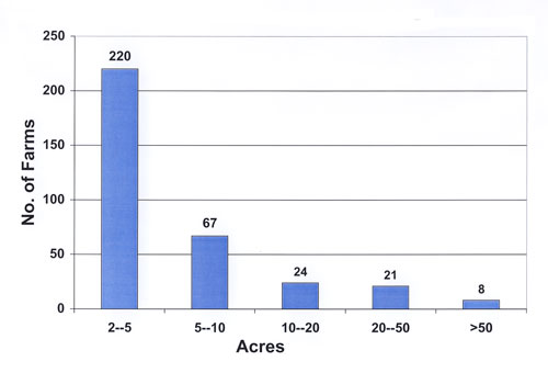
Figure 1. Pecan farm or parcel size distribution, 2001, n = 340.
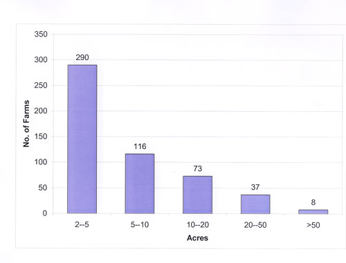
Figure 2. Alfalfa farm or parcel size distribution, 2001, n = 524.
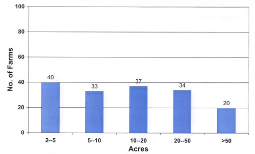
Figure 3. Cotton farm/parcel size distribution, 2001, n = 164.
All analysis of the data was conducted using Excel™ spreadsheet and SAS™ statistical analysis software. Data were sorted and analyzed by crop, by parcel size, by irrigation duration, by water applied, by time of irrigation, and other variables provided by EBID. The results of the data analysis are presented here in figures and tables.
Almost two-thirds of the pecan farms and 55% of the alfalfa farms analyzed were irrigating less than five acres, while the distribution of cotton farms was more even across the acreage categories. The data cover 2,716 acres of pecans, 4,036 acres of alfalfa and 3,390 acres of cotton. The data received from EBID represent approximately 13% of total pecan acreage in the district, about 15% of alfalfa acreage and about 20% of cotton acreage. Because there were so few farms in the largest farm size category (>50 acres), all observations larger than or equal to 20 acres were put in the same farm size group for the analyses discussed below.
Findings
Prior to data analysis, it was hypothesized that differences in amounts of irrigation water applied and time spent irrigating would exist between farms of different sizes. Differences in soil types and on-farm irrigation water turnouts also were assumed to be factors that would influence water applied and time spent irrigating. Findings are discussed below relative to the irrigation variable considered and by crop.
Total Irrigation Water Applied
Figure 4 presents acre-feet/acre of water applied to pecans relative to farm size, and shows a wide range of water applied per acre for all farm sizes. The quantities of water are based on the district's estimates of how much water went onto the parcels for which water was requested, which is a function of previous engineering estimates of canal deliveries.
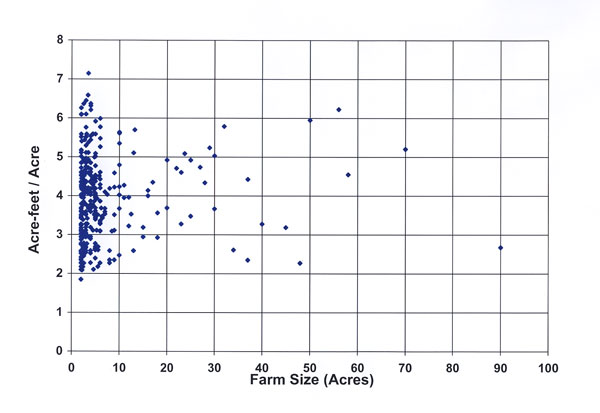
Figure 4. Pecan acre-feet per acre water applied by farm size (2001, n = 340).
As might be expected from observation of fig. 4, the pecan acre-feet/acre means for total water applied were not dramatically different across the farm size acreage groups. Descriptive statistics and quantile analysis for acre-feet/acre of water applied for the 340 pecan farms are presented in table 2. Analysis of variance confirmed that the water applied means were not significantly different; however, the range of water applied does vary greatly by farm size. The range of water applied across all quantiles is 5.30 acre-feet/acre for the smallest farm size, which is larger than the other farm size categories. The irrigation district data included no information about supplemental groundwater, and parcels which received surface water less than five times during the irrigation season were not included in the analysis in an effort to eliminate farms which apply primarily groundwater. Nevertheless, it is curious to see the low levels of surface water applications in the 25% of the pecan farms using the least amount of water in each farm size category. It may thus be more appropriate to compare the ranges of water applied to pecans for the highest 25% of water users in each farm size category to reduce the likelihood of supplemental groundwater use. Examination of the ranges of water applied for the highest 25% of water users again shows the largest range of acre-feet/acre water applied in the smallest farm size group.
Table 2. Quantile analysis and descriptive statistics for pecan water applied (acre-feet/acre) relative to farm size (2001, n = 340).
| Farm Size Category | |||||
| Quantiles | 2 ≤ acres < 5 | 5 ≤ acres < 10 | 10 ≤ acres < 20 | ≥ 20 acres | |
| 0% | Minimum acre-fee/acre water applied | 1.85 | 2.18 | 2.47 | 2.27 |
| 25% | 3.04 | 3.11 | 3.37 | 3.28 | |
| 50% | Median acre-fee/acre water applied | 3.78 | 3.67 | 4.01 | 4.49 |
| 75% | 4.53 | 4.37 | 4.95 | 4.98 | |
| 80% | 4.72 | 4.51 | 5.35 | 5.09 | |
| 85% | 4.97 | 4.61 | 5.61 | 5.20 | |
| 90% | 5.44 | 5.09 | 5.63 | 5.79 | |
| 95% | 6.09 | 5.59 | 5.64 | 5.95 | |
| 99% | 6.45 | 5.99 | 5.70 | 6.23 | |
| 100% | Maximum acre-feet/acre water applied | 7.15 | 5.99 | 5.70 | 6.23 |
| Descriptive Information | |||||
| Number of farms | 223 | 65 | 24 | 28 | |
| Percent farms | 65.6 | 19.1 | 7.1 | 8.2 | |
| Mean acre-feet/acre1 | 3.91 | 3.79 | 4.12 | 4.23 | |
| Grand mean – all farm size groups | 3.93 acre-feet/acre (47.16 inches/acre) | ||||
| Standard deviation (acre/feet/acre) | 1.05 | 0.94 | 0.99 | 1.09 | |
| Range (all quantiles) (acre-feet/acre) | 5.30 | 3.81 | 3.23 | 3.96 | |
| Range (75% – 100%) (acre-feet/acre) | 2.62 | 1.62 | 0.75 | 1.25 | |
| Number of acres | 648 | 396 | 303 | 1,368 | |
| Percent acres | 23.9 | 14.6 | 11.2 | 50.4 | |
| Total water applied (acre-feet) | 2,567 | 1,483 | 1,224 | 5,748 | |
| Percent total water applied | 23.4 | 13.4 | 11.1 | 52.2 | |
| 1Means were not significantly different. | |||||
Table 2 also shows the number of acres and the percentage of total acres in each farm size category for the 340 observations for which data were analyzed. The acre-feet of water applied in each farm size category and percentages of total water applied in all farm size categories (according to the EBID data) are also presented in table 2. The similarities in the numbers for "percent acres" and "percent water applied" will be discussed later in this report.
Acre-feet/acre of water applied to alfalfa parcels relative to farm size is presented in fig. 5. Figure 5 exhibits a pattern similar to that of pecans (fig. 4); however, analysis of variance found significant differences in means of water applied for alfalfa. Specifically, the mean acre-feet/acre for the smallest farm size was significantly lower than the means for farms in the 10 ≤ acres < 20 and ≥ 20 acres groups (table 3). As presented in table 3, differences in the ranges of water applied for the highest 25% of water users are very large, with an almost 10-fold difference between the smallest and largest farm size groups. The most extreme observations of the highest water users are not shown in fig. 5, although they were included in the analysis presented in table 2. A simple examination of differences in mean water applied by farm size indicates that larger parcels have a higher average level of water applied. However, the data for ranges of water applied complicate that conclusion, and show that even when the highest 1% of extreme observations is excluded, the range of water applied is greatest for the smallest farm size. Thus, given the large number of smaller parcels (2 ≤ acres < 5 parcels are 55% of all alfalfa parcels analyzed), the cumulative amount of water applied by the highest 25% of alfalfa water users is quite large. As with the pecan water application data, information for acres, percentage of total acres, water applied, and percentage of total water applied is also presented in table 3 for the different size groups.
Table 3. Quantile analysis and descriptive statistics for alfalfa water applied (acre-feet/acre) relative to farm size (2001, n = 524).
| 1 | Farm Size Category | ||||
| Quantiles | 2 ≤ acres < 5 | 5 ≤ acres < 10 | 10 ≤ acres < 20 | ≥ 20 acres | |
| 0% | Minimum acre-fee/acre water applied | 2.00 | 2.19 | 2.29 | 2.21 |
| 25% | 3.03 | 3.39 | 3.76 | 3.90 | |
| 50% | Median acre-fee/acre water applied | 3.86 | 4.17 | 4.45 | 4.62 |
| 75% | 4.75 | 4.98 | 5.37 | 5.14 | |
| 80% | 5.08 | 4.17 | 5.50 | 5.75 | |
| 85% | 5.34 | 5.31 | 5.76 | 6.00 | |
| 90% | 5.61 | 5.59 | 5.99 | 6.13 | |
| 95% | 6.13 | 6.59 | 6.59 | 6.54 | |
| 99% | 8.55 | 7.19 | 7.25 | 6.59 | |
| 100% | Maximum acre-fee/acre water applied | 19.18 | 10.91 | 7.25 | 6.59 |
| Descriptive Information | |||||
| Number of farms | 290 | 116 | 73 | 45 | |
| Percent farms | 55.3 | 22.1 | 13.9 | 8.6 | |
| Mean acre-fee/acre1 | 4.06ab | 4.29 | 4.52a | 4.60b | |
| Grand mean – all farm size groups | 4.22 acre-feet/acre (50.64 inches/acre) | ||||
| Standard deviation (acre/feet/acre) | 1.53 | 1.24 | 1.11 | 1.11 | |
| Range (all quantiles) (acre-feet/acre) | 17.18 | 8.72 | 4.96 | 4.38 | |
| Range (75% – 100%) (acre-feet/acre) | 14.43 | 5.93 | 1.88 | 1.45 | |
| Number of acres | 884 | 727 | 946 | 1,479 | |
| Percent acre | 21.9 | 18.0 | 23.4 | 36.7 | |
| Total water applied (acre-feet) | 3,605 | 3,117 | 4,363 | 6,734 | |
| Percent total water applied | 20.2 | 17.5 | 24.5 | 37.8 | |
| 1Means with the same letter are significantly different at p < 0.05 | |||||
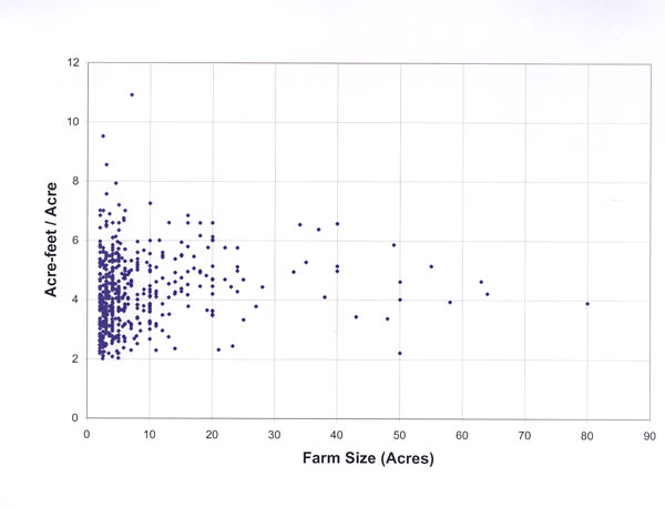
Figure 5. Alfalfa acre-feet per acre water applied by farm size (2001, n = 524).
Figure 6 shows acre-feet/acre of water applied by farm size for cotton parcels. Quantile analysis and descriptive statistics for water applied to cotton are presented in table 4. Analysis of variance found no significant differences in mean water applied to cotton parcels. The range of water applied across all quantiles and across the highest 25% of water users is greatest for the largest farm group (i.e., farm size of at least 20 acres). These results are very different from those found for pecans and alfalfa. The distribution of cotton parcels is more heavily weighted toward larger parcels than either pecans or alfalfa (see figs. 1-3), and the total number of cotton observations is small relative to the other two crops. As with the pecan and alfalfa data, percentage of total acres and percentage of total water applied for cotton presented in table 4 are similar.
Table 4. Quantile analysis and descriptive statistics for cotton water applied (acre-feet/acre) relative to farm size (2001, n = 164).
| Farm Size Category | |||||
| Quantiles | 2 ≤ acres < 5 | 5 ≤ acres < 10 | 10 ≤ acres < 20 | ≥ 20 acres | |
| 0% | Minimum acre-fee/acre water applied | 2.18 | 1.89 | 1.79 | 1.94 |
| 25% | 2.28 | 2.35 | 2.27 | 2.27 | |
| 50% | Median acre-feet/acre water applied | 2.35 | 2.43 | 2.35 | 2.40 |
| 75% | 2.71 | 2.69 | 2.69 | 2.70 | |
| 80% | 2.77 | 2.73 | 2.85 | 2.77 | |
| 85% | 2.86 | 2.90 | 2.85 | 2.77 | |
| 90% | 2.93 | 2.94 | 3.17 | 2.88 | |
| 95% | 3.09 | 3.04 | 3.19 | 3.20 | |
| 99% | 3.27 | 3.19 | 3.20 | 4.83 | |
| 100% | Maximum acre-feet/acre water applied | 3.27 | 3.19 | 3.20 | 4.83 |
| Descriptive Information | |||||
| Number of farms | 40 | 33 | 37 | 54 | |
| Percent farms | 24.4 | 20.1 | 22.6 | 32.9 | |
| Mean acre-feet/acre1 | 2.53 | 2.52 | 2.47 | 2.54 | |
| Grand mean – all farm size groups | 2.52 acre-feet/acre (30.24 inches/acre) | ||||
| Standard deviation (acre/feet/acre) | 0.29 | 0.30 | 0.35 | 0.47 | |
| Range (all quantiles) (acre-feet/acre) | 1.09 | 1.30 | 1.41 | 2.89 | |
| Range (75% – 100%) (acre-feet/acre) | 0.99 | 0.50 | 0.51 | 2.13 | |
| Number of acres | 119 | 241 | 525 | 2,505 | |
| Percent acres | 3.5 | 7.1 | 15.5 | 73.9 | |
| Total water applied (acre-feet) | 298 | 607 | 1,297 | 6,130 | |
| Percent total water applied | 3.6 | 7.3 | 15.6 | 73.6 | |
| 1Means were not significantly different. | |||||
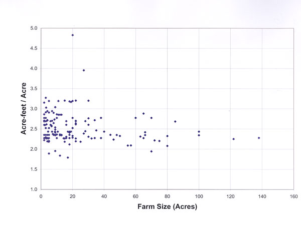
Figure 6. Cotton acre-feet per acre water applied by farm size (2001, n = 164).
Comparison of EBID Water Delivery Data to Derived Consumptive Use
The average amount of water applied to pecans, alfalfa and cotton in the area served by EBID can be derived using average county-yield data for the three crops. The results of the derived water application analysis can be compared to the average water application estimates which were calculated using EBID's data and reported in this document. Yield is directly related to crop water consumptive use or evapotranspiration (ET) through crop water production functions which have been developed for southern New Mexico by various investigators. Table 5 presents crop water production functions for pecans, alfalfa and cotton, all in metric units because the original research and publications employed metric units.
Table 5. Crop water production functions for various crops in southern New Mexico. Y is yield in metric ton/ha and ET is seasonal evapotranspiration in cm (Samani et al., 2004).
| Water Production Function | Crop | Reference |
| Y = (-30.1 + 22.14*ET)/1000 | Pecan | Miyamoto, 1983 |
| Y = 0.14 + 0.12*ET | Alfalfa | Sammis, 1981 |
| Y = (134.87 + 14.25*ET)/1000 | Cotton | Sammis, 1981 |
If estimates of irrigation efficiency are available, then average applied water can be derived from linking crop yields to the following relationship: Applied water = ET/Efficiency, where "ET" is evapotranspiration and "Efficiency" is on-farm irrigation efficiency. Samani et al. (2004) used the chloride tracing technique to measure on-farm irrigation efficiency (defined as ET/total applied water) on selected commercial farms. On-farm irrigation efficiencies for the sampled farms' pecans, alfalfa and cotton were estimated as 93.2%, 93% and 95%, respectively (Samani et al., 2004). Ten-year average Doña Ana County yields for the period 1993-2002 (published in New Mexico Agricultural Statistics) were used to derive ET and applied water for the three crops as shown in table 6.
Table 6. Derived average evapotranspiration (ET) for pecans, alfalfa, and cotton.
|
Average county yield |
Derived ET, |
On-farm irrigation efficiency % |
Derived total applied water, cm/year |
EBID average applied water |
|
| Crop | [New Mexico Agricultural Statistics, 2004] | [Calculated from yield functions Table 5, this report] | [Samani et al., 2004] | [Calculated: Applied water = ET/Efficiency] | [From Tables 2, 3, 4, this report] |
| Pecans | 1.62 mt/ha (1,448 lbs/ac) |
74.67 cm (29.40 in) |
93.2% | 80.11 cm (31.54 in) |
119.79 cm (47.16 inches) |
| Alfalfa | 15.83 mt/ha (7.06 T/ac) |
130.72 cm (51.47 in) |
93% | 140.55 cm (55.34 in) |
128.63 cm (50.64 inches) |
| Cotton | 1.09 mt/ha (1,402 lbs/ac) |
66.75 cm (26.28 in) |
95% | 70.23 cm (27.65 in) |
76.81 cm (30.24 inches) |
On-farm irrigation efficiencies estimated using the chloride method include the effect of both irrigation water and rainfall. Average annual rainfall in the area served by EBID is 8 inches (20 cm). If it is assumed that 50% of rainfall is effective, then the amount of irrigation water applied can be estimated by subtracting effective rainfall from total applied water as shown in table 7.
Table 7. Derived average applied irrigation water for pecans, alfalfa and cotton.
| Derived applied irrigation water (excluding rainfall) | EBID average applied water, cm/year | Percent difference | |
| cm/year (inches/year) | cm/year (inches/year) | Calculated: | |
| From yield functions, see table 6, this report. | From EBID data, see tables 2, 3 and 4, this report. | ||
| Crop | (A) | (B) | [(B – A)/ A]*100 |
| Pecans | 70.11 cm (27.60 inches) | 119.79 cm (47.16 inches) | +70.86% |
| Alfalfa | 130.55 cm (51.40 inches) | 128.63 cm (50.64 inches) | -1.47% |
| Cotton | 60.23 cm (23.72 inches) | 76.81 cm (30.24 inches) | +27.53% |
The comparison of results for derived applied irrigation water (excluding rainfall), and EBID average applied water in table 7 above shows that applied irrigation water estimated from average county yield is remarkably close to EBID average records for alfalfa (-1.47% difference). District records show 70.86% more water applied to pecans and 27.53% more water applied to cotton, than were derived using county average yields and yield functions. County average yields are calculated from estimates of total production and total acreage. From table 7, it can be tentatively concluded that yields calculated using this method are lower than the yields achieved by many (commercial) producers. The large positive differences may also reflect low harvest indices. The harvest index is the ratio of yield to total annual biomass production (Sinclair, 1998). If pecans and cotton are not intensively managed with yield objectives in mind, irrigation water will produce biomass (i.e., leaves) but not necessarily increase nut or lint yields. Also, yield values obtained from the producers who participated in the chloride tracing research tended to be higher than the 10-year average yields presented in table 6 (Samani et al., 2004).
The results in table 7 for pecans and cotton also lead to doubts about existing levels of on-farm irrigation efficiencies across the wide range of farms. As stated above, the on-farm efficiency estimates presented in table 6 were for larger, commercial farms. The number of acres irrigated with these high efficiencies contributes to the relatively high average district on-farm efficiency reported in table 1. If the average on-farm efficiency used in the table 6 calculations drops to 62% for pecans and 87% for cotton (and the county average yields are again used), then the derived ET is more consistent with EBID's records of average applied water.
The alfalfa results support the observation that average on-farm irrigation efficiency in the study region is high and that average water applied to alfalfa conforms to estimated water applied (based on reported yields). Also, with alfalfa there is a very high correlation between yield and biomass production. As shown in table 3 there is a wide range of water application levels within farm size groups, and there is potential for reducing water use by farmers who are over applying. However, if every alfalfa irrigator were to apply an equal amount of water, then the potential for net water saving at the farm level is marginal given the situation illustrated by the 2001 data, where heavy irrigation by some water users is offset by extreme deficit or under-irrigation by other irrigators.
The random field measurements conducted in the course of this research showed that, for alfalfa irrigators, the EBID accounting of billed water is about 30-35% lower than field measured applications. For cotton, field measurements indicate that EBID accounting of water applied is ~10% lower than applied water. For pecans, water applied was found to be more consistent with EBID's records for the farms where field measurements were taken. This does not mean that any of these irrigators have lower or higher on-farm application efficiencies. Rather, some of the irrigators who are applying more water than they are being charged for may have high efficiencies which result in higher yields, or low efficiencies and low yields. Other irrigators who are under-applying are paying for more water than they are receiving, and could have either high or low efficiencies and high or low yields.
As noted above, EBID conveyance efficiency (i.e., diversion / farm delivery) is reported to be 54%. This research identified numerous instances of overdelivery onto farms. These field observations lead to doubts about the accuracy of the 54% conveyance efficiency. If numerous farmers are undercharged (i.e., overdelivered), then this leads us to question the current estimates of conveyance losses in the EBID delivery system, and to speculate that some of this water is instead applied to crops.
Irrigation Duration
As indicated above, the district's 2001 accounting of water delivered does not reflect measurements in the field. The water delivery data analyzed are based on engineering estimates of canal deliveries. During examination of the 2001 water delivery data provided by EBID, differences in irrigation durations between farms became very obvious. The EBID data included start and stop times for water deliveries, and spreadsheet functions were used to estimate total irrigation durations and irrigation durations per acre. Irrigation duration (i.e., hours/acre/irrigation) is an indicator of field level irrigation efficiency, and is particularly useful when measurements of water applied are unreliable.
A long duration can be caused by several factors, including lack of attention to irrigation practices, lack of knowledge of crop consumptive water requirements, highly permeable soils, small and/or unlined farm ditches, small farm turnouts, several users on a single delivery ditch attempting to irrigate simultaneously, and low water discharge at the farm turnout. The low discharge can be due to both poor water delivery infrastructure at the farm turnout and insufficient flows, a single factor, or a combination of several factors. Prior field work and recent observations throughout the district by the authors have resulted in the empirical guideline of 0.5 hours/acre/irrigation. Regardless of soil type (e.g., sand, loam, clay), it has been found that irrigations on large, commercially oriented farms typically require about 30 minutes of water flow per acre through the farm turnout onto the field. This guideline reflects typical lengths of run for the water in the fields, normal water flows at the farm turnouts, and adequately sized on-farm turnouts. On heavy, clay soils, 0.2 hours/acre/irrigation has been observed. Very long irrigations usually indicate that on-farm irrigation efficiency will be reduced as a result of deep percolation losses at the front end of the field.
Figure 7 shows the relationship between duration of irrigation and farm size for the pecan farms (n = 340) analyzed. The figures reveal large differences in irrigation duration between small and large farms. The scale of this figure has also been adjusted such that several extreme data points in the range of 12-26 hours/acre/ irrigation are not shown on the figure, although those data were included in the quantile analysis presented in table 8. Figures 8 and 9 present irrigation durations versus farm size for alfalfa (n = 524) and cotton (n = 164), respectively. All three figures exhibit the same pattern, with irrigation duration dropping off dramatically at approximately 20 acres, and remaining close to the empirical guideline of 0.5 hours/acre/irrigation for larger farm sizes. The pattern is very similar for pecans and alfalfa, with cotton showing more variability at the larger farm sizes.
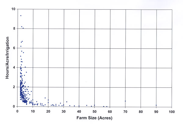
Figure 7. Pecan hours per acre per irrigation vs. farm size (2001, n = 340).
Figure 8. Alfalfa hours per acre per irrigation vs. farm size (2001, n = 524).
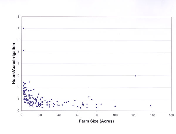
Figure 9. Cotton hours per acre per irrigation vs. farm size (2001, n = 164).
Average hours per acre per irrigation are shown by acreage category in figs. 10, 11 and 12 for pecans, alfalfa and cotton. Descriptive statistics and quantile analysis for irrigation durations are presented in tables 8, 9 and 10 for the three crops.
As expected from examination of figures 10, 11 and 12, mean irrigation durations are greatest for the smallest farms, and decline with increasing farm size. Large differences in mean irrigation duration exist across farm size groups for all three crops. The statistically significant differences in means are noted in tables 8, 9 and 10. The very large differences in the ranges of irrigation durations (across all quantiles, and for the longest 25% of irrigations) are also presented in tables 8, 9 and 10. Differences in irrigation durations and ranges between the 2 ≤ acres < 5 group and all other farm size groups are very striking. There is a clear distinction in irrigation duration on parcels of less than five acres relative to all other parcel sizes. The pecan, alfalfa and cotton data sets also were each divided into four equal quartiles by hours/acre/irrigation, and chi-square tests of differences in proportions were conducted. The chi-square analyses found that for every crop, there were significantly more small farms with the longest irrigation durations, and significantly more large farms with the shortest irrigation durations.
Table 8. Quantile analysis and descriptive statistics for pecan irrigation durations (hours/acre/irrigation) relative to farm size (2001, n = 340).
| Farm Size Category | |||||
| Quantiles | 2 ≤ acres < 5 | 5 ≤ acres < 10 | 10 ≤ acres < 20 | ≥ 20 acres | |
| 0% | Minimum hours/acre/irrigation | 0.35 | 0.46 | 0.28 | 0.91 |
| 25% | 0.98 | 0.70 | 0.52 | 0.28 | |
| 50% | Median hours/acre/irrigation | 1.25 | 0.82 | 0.65 | 0.38 |
| 75% | 1.71 | 1.17 | 0.92 | 0.46 | |
| 80% | 1.80 | 1.24 | 0.97 | 0.53 | |
| 85% | 1.95 | 1.48 | 1.01 | 0.53 | |
| 90% | 2.14 | 1.65 | 1.40 | 0.81 | |
| 95% | 2.73 | 1.74 | 1.44 | 0.83 | |
| 99% | 7.54 | 2.05 | 2.01 | 1.09 | |
| 100% | Maximum hours/acre/irrigation | 25.6 | 2.05 | 2.01 | 1.09 |
| Descriptive Information | |||||
| Number of farms | 223 | 65 | 24 | 28 | |
| Mean hours/acre/irrigation1 | 1.57abc | 0.97a | 0.76b | 0.42c | |
| Grand mean – all farm size groups | 1.30 hours/acre/irrigation | ||||
| Standard deviation (hours/acre/irrigation) | 1.93 | 0.40 | 0.40 | 0.21 | |
| Range (all quantiles) (hours/acre/irrigation) | 25.25 | 1.59 | 1.73 | 0.90 | |
| Range (75% - 100%) (hours/acre/irrigation) | 23.89 | 0.71 | 0.64 | 0.63 | |
| Total irrigation hours | 10,288 | 4,165 | 1,473 | 2,004 | |
| Percent total irrigation hours | 57.4 | 23.2 | 8.2 | 11.2 | |
| 1Means with the same letter are significantly different at p < 0.05 | |||||
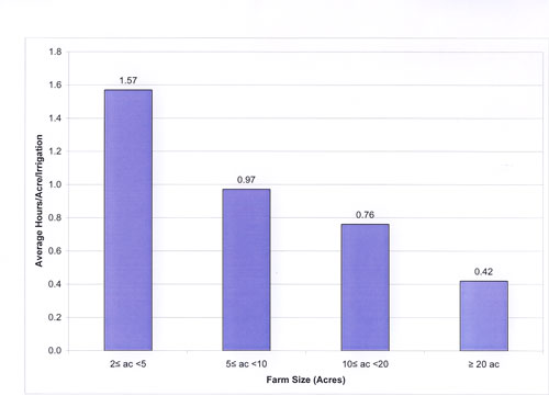
Figure 10. Pecan average hours/acre/irrigation (2001, n = 340)
Table 9. Quantile analysis and descriptive statistics for alfalfa irrigation durations (hours/acre/irrigation) relative to farm size (2001, n = 524).
| Farm Size Category | |||||
| Quantiles | 2 ≤ acres < 5 | 5 ≤ acres < 10 | 10 ≤ acres < 20 | ≥ 20 acres | |
| 0% | Minimum hours/acre/irrigation | 0.59 | 0.44 | 0.33 | 0.24 |
| 25% | 1.10 | 0.72 | 0.56 | 0.46 | |
| 50% | Median hours/acre/irrigation | 1.38 | 1.00 | 0.74 | 0.55 |
| 75% | 1.86 | 1.33 | 1.12 | 0.67 | |
| 80% | 2.06 | 1.39 | 1.19 | 0.70 | |
| 85% | 2.29 | 1.52 | 1.29 | 0.74 | |
| 90% | 2.73 | 1.76 | 1.50 | 0.90 | |
| 95% | 3.92 | 2.25 | 2.27 | 0.99 | |
| 99% | 7.20 | 2.55 | 2.83 | 1.09 | |
| 100% | Maximum hours/acre/irrigation | 9.90 | 2.76 | 2.83 | 1.09 |
| Descriptive Information | |||||
| Number of farms | 290 | 116 | 73 | 45 | |
| Mean hours/acre/irrigation1 | 1.73abc | 1.10ad | 0.92be | 0.57cde | |
| Grand mean – all farm size groups | 1.38 hours/acre/irrigation | ||||
| Standard deviation (hours/acre/irrigation) | 1.19 | 0.50 | 0.53 | 0.20 | |
| Range (all quantiles) (hours/acre/irrigation) | 9.31 | 2.32 | 2.50 | 0.85 | |
| Range (75% - 100%) (hours/acre/irrigation) | 8.04 | 1.43 | 1.71 | 1.02 | |
| Total irrigation hours | 11,836 | 6,870 | 8,077 | 8,070 | |
| Percent total irrigation hours | 33.9 | 19.7 | 23.2 | 23.2 | |
| 1Means with the same letter are significantly different at p < 0.05 | |||||
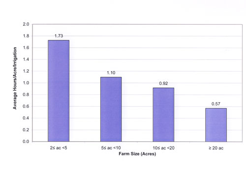
Figure 11. Alfalfa average hours/acre/irrigation (2001, n = 524)
Table 10. Quantile analysis and descriptive statistics for cotton irrigation durations (hours/acre/irrigation) relative to farm size (2001, n = 164).
| Farm Size Category | |||||
| Quantiles | 2 ≤ acres < 5 | 5 ≤ acres < 10 | 10 ≤ acres < 20 | ≥ 20 acres | |
| 0% | Minimum hours/acre/irrigation | 0.68 | 0.39 | 0.35 | 0.24 |
| 25% | 1.17 | 0.76 | 0.53 | 0.47 | |
| 50% | Median hours/acre/irrigation | 1.56 | 0.92 | 0.70 | 0.55 |
| 75% | 1.94 | 1.25 | 0.94 | 0.78 | |
| 80% | 2.13 | 1.31 | 1.01 | 0.89 | |
| 85% | 2.28 | 1.68 | 1.13 | 0.92 | |
| 90% | 2.40 | 1.74 | 1.31 | 0.98 | |
| 95% | 3.75 | 1.80 | 1.71 | 1.11 | |
| 99% | 7.00 | 2.43 | 1.78 | 2.97 | |
| 100% | Maximum hours/acre/irrigation | 7.00 | 2.43 | 1.78 | 2.97 |
| Descriptive Information | |||||
| Number of farms | 40 | 33 | 37 | 54 | |
| Mean hours/acre/irrigation1 | 1.76abc | 1.05ad | 0.77b | 0.67cd | |
| Grand mean – all farm size groups | 1.03 hours/acre/irrigation | ||||
| Standard deviation (hours/acre/irrigation) | 1.13 | 0.44 | 0.35 | 0.40 | |
| Range (all quantiles) (hours/acre/irrigation) | 6.33 | 2.05 | 1.44 | 2.73 | |
| Range (75% - 100%) (hours/acre/irrigation) | 5.06 | 1.18 | 0.84 | 2.19 | |
| Total irrigation hours | 1,008 | 1,356 | 2,123 | 9,697 | |
| Percent total irrigation hours | 7.1 | 9.6 | 15.0 | 68.4+ | |
| 1Means with the same letter are significantly different at p < 0.05 | |||||
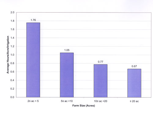
Figure 12. Cotton average hours/acre/irrigation (2001, n = 164)
Several fields with long irrigation durations were visited during the 2002 and 2003 irrigation seasons to gain a better understanding of the conditions which led to the lengthy irrigation periods, and to confirm whether the extreme observations found in the EBID data were accurate representations of on-farm conditions. These fields were visited while irrigations were underway. Fields with average and below average irrigation durations were also visited while irrigations were occurring in order to compare those conditions with long duration conditions.
Common reasons identified for long durations were the condition of the farm delivery ditches and the size of the on-farm turnouts. In several cases, the water was moving so slowly through the farm delivery ditches toward the on-farm turnouts that flow measurements could not be taken with a digital propeller meter. The water was released from the district's larger canal via partially open 24-inch gates into the farm delivery ditch, and then through very small on-farm turnouts onto the fields. These small turnouts were usually round 4-inch pipes. In other cases, the on-farm turnouts were not really structures; instead, they were more like controlled breaks in the farm delivery ditch. When asked about the length of time spent irrigating their fields, several individuals complained about the bad condition of the on-farm delivery ditch from which they take their water. The irrigation district has no responsibility or authority for maintaining these ditches, and the irrigators noted that weeds, trash, rodents and breaks were factors that resulted in long irrigation durations. In the case of one of the long-duration fields, a fallow lot approximately 100 feet wide and 100 feet long was being used as a channel through which the water flowed uncontrolled before it reached the small pecan orchard actually being irrigated. Complaints about neighbors' unwillingness to grant easements for improving irrigation water delivery or allow modifications to easements for the purpose of increasing the size of the on-farm delivery infrastructure were often heard.
Conversations with the irrigators conducted during the field visits revealed some common themes. One theme can be summarized by an older man's comment regarding the fact that it took him almost two days to irrigate his ~3 acre pecan orchard. He said, "I'm retired, what else have I got to do?" Other comments revolved around the view that irrigation was a family tradition, that irrigating often meant the involvement of members of extended families, that irrigation was a social undertaking, that irrigation was a peaceful, meditative, enjoyable task.
Overall, the levels of irrigation technology and water management found on field visits to small farms were extremely low, and often a consequence of inadequate irrigation design. The principal design problem found was narrow diameter farm turnouts which cannot physically deliver to the field the minimum flow necessary to rapidly push the water across the field, thus reducing both the time spent irrigating and infiltration losses during the irrigation process. The level of involvement by other small-scale water users in the practice of irrigation also appeared to be quite low, and a relatively high degree of resentment toward other users of the same farm delivery ditches was noted among some interviewees (e.g., "Nobody else does anything to maintain the ditch, why should I?"). Many of the long-duration irrigators complained about their neighbors' unwillingness to improve the mutual on-farm delivery ditch (i.e., that part of the delivery system not maintained by the district).
Field data obtained from the observed irrigations during the 2002 and 2003 irrigation seasons were used to estimate water deliveries onto the farms and compare these estimates with those recorded by EBID (presented in figs. 4-6 and tables 8-10 above). The EBID water delivery data were collected for the objective of billing irrigators, and were not the result of measurements of on-farm deliveries. Results of the field measurements have been intriguing, and usually at odds with the district's water delivery data, which record six acre-inch deliveries for most irrigation events. Field analysis on selected farms consistently found that the amount of water applied to a field is strongly and positively related to irrigation duration per acre. Irrigation depths per event ranging from 2.2 acre-inches to 14.7 acre-inches were measured in fields. Furthermore, the excessively high water applications (including the 14.7 acre-inch case cited above) are an average across the entire parcel, and do not account for what may be 20+ acre-inch infiltrations at the top of the fields. These high top-end applications occur during the process of the irrigation water's slow advance to the bottom of the fields.
Results of the field measurements taken in 2002 and 2003 indicated a large range of water deliveries to farms, and some patterns have emerged. Results have tended to show underdelivery (i.e., less than six acre-inches) and subsequent overcharges to larger fields, while smaller fields (i.e., less than 10 acres) tend to receive more than six acre-inches per irrigation. Smaller farms are thus undercharged for their irrigation water. Overdelivery of water is related to the excessively long irrigation durations discussed above, with reasons for overdelivery including long fields (i.e., irrigation runs in excess of 1,200 feet), rough field surfaces, low flows and small turnouts to the farm. During field work many water deliveries ranging from eight to 12 acre-inches were measured. The fields receiving the water were generally smaller, although not exclusively so. Many deliveries in the range of two to four acre-inches on larger fields were also measured. These fields tended to be intensively managed (evidenced by surface smoothness and absence of weeds), and were part of large, commercial farming operations. These fields also tended to be located near the larger delivery canals, irrigated through large turnouts, and received high flows of water during the observed irrigation events. The water rapidly moved across the fields, and due to the common practice of shutting off the water when it reaches the end of the field, underdelivery occurred. Prior to this research effort, in the process of testing flumes and training students in their use, the authors also found underdelivery of irrigation water to larger farms.
Monthly Irrigations and Evapotranspiration
Both field work and examination of the irrigation district's data also lead to the conclusion that there is generally little relationship between seasonal water demand and applied water for the fields studied. Lack of knowledge about and inattention to irrigation scheduling based on crop water demands contribute to low on-farm water use efficiency. Traditional irrigation timing practices (i.e., every 7-14 days throughout the irrigation season) contribute to overwatering at the beginning and end of the irrigation season, plant stress at peak crop water use periods, and can result in reductions in both crop yields and quality. Figures 13 and 14 show average water applied by month for each farm size group on the left vertical axes, and maximum monthly evapotranspiration plotted on the right vertical axes.
The pattern of water application to pecans and alfalfa is similar across the different farm size groups. Average acre-feet/acre/month applied to pecans is very stable throughout the irrigation season, while alfalfa generally shows decreasing applications from the beginning to the end of the irrigation season. Both figures 13 and 14 illustrate heavy irrigation at the beginning of the irrigation season. Figure 13 shows less than optimal applications to pecans during the peak growing months of June and July. For all the alfalfa farm sizes, irrigation water applied at the end of the season (i.e., September and October) is higher than maximum evapotranspiration.
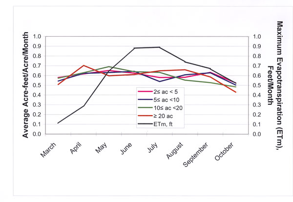
Figure 13. Pecan average acre-feet/acre/month water applied by farm size (by month, 2001, n = 340) and maximum evapotranspiration.
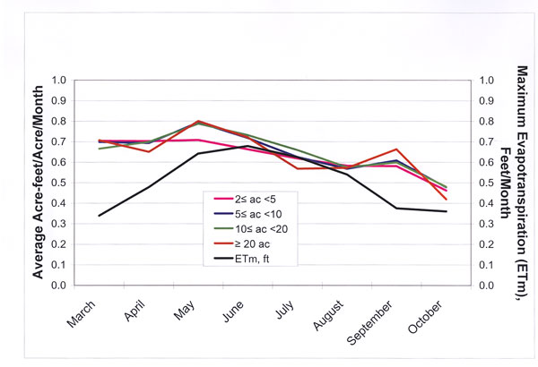
Figure 14. Alfalfa average acre-feet/acre/month water applied by farm size (by month, 2001, n = 524) and maximum evapotranspiration.
Irrigation management in cotton involves striking a balance between excessive foliage growth due to abundant water in the root zone and reduced yields due to limited water availability (Milroy, Goyne and Larsen, 2002). Optimal cotton production is achieved when the cotton plant is subjected to some drought stress to keep leaf development under control, but not to the point of reducing yields. Thus, while potential maximum cotton evapotranspiration rises in the spring, growers dramatically reduce water applied to cotton, as illustrated in fig. 15. Figure 15 also shows a very similar pattern of water applied to cotton for all farm size groups. Deficit irrigation practices are very obvious in fig. 15 from July through the end of the growing season.
Additional insight into irrigation practices is given in figs. 16, 17 and 18, which show the differences in irrigation durations for the different farm size groups. In these figures, average hours/acre/month irrigation duration is plotted on the left vertical axes. As stated above, the EBID data are based on engineering estimates with six acre-inches recorded for most deliveries; field measurements are not consistent with the water delivery data. Again, this research has found a strong, positive relationship between irrigation duration and water applied.
Irrigation durations for pecans are shown to be very consistent from March to October for the smallest size farms (2 ≤ acres < 5), and relatively little variability in irrigation duration for the other three farm size groups. When maximum evapotranspiration is steeply increasing during April and May, many pecan irrigators are reducing their irrigation durations (e.g., 5 ≤ acres < 10; ≥ 20 acres). Alfalfa irrigation durations vary widely across the farm size groups, decreasing in the early summer for the three larger farm size groups (at the same time that ETm increases), and increasing in the late summer (as ETm drops off). Cotton irrigation durations increase for the smallest farm size group during May, while the other farm size groups reduce duration (with no May irrigation events for the 10 ≤ acres < 20 group).
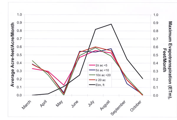
Figure 15. Cotton average acre-feet/acre/month water applied by farm size (by month, 2001, n = 164).
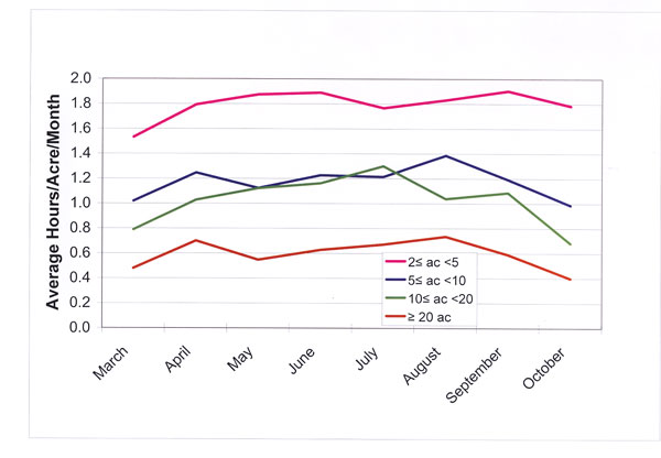
Figure 16. Pecan average irrigation duration by farm size (by month, 2001, n = 340)
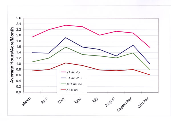
Figure 17. Alfalfa average irrigation duration by farm size (by month, 2001, n = 524).
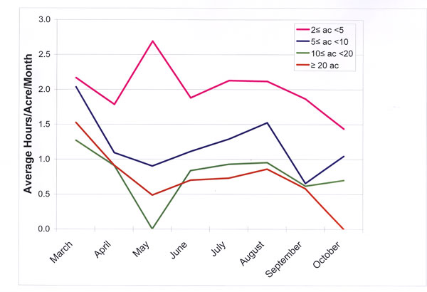
Figure 18. Cotton average irrigation duration by farm size (by month, 2001, n = 164)
Cumulative Distribution of Total Water Applied and Total Irrigation Hours
The cumulative distribution of total water applied relative to total acreage irrigated was examined for pecans, alfalfa and cotton and are presented here using Lorenz Curves. Figures 19, 20 and 21 illustrate the impact of the engineering assumption of a six-inch/acre water delivery when the observations are sorted by smallest to largest farm size group. Figure 19 presents the cumulative distribution of water across the 2,715 acres of pecans represented in the EBID data. If the data showed a perfectly equal distribution of water across all the irrigated acres from the smallest to the largest farms, there would be no area between the 45-degree line (i.e., the Line of Equal Distribution) and the Lorenz curve (in red). Figure 19 shows very little area between the two lines. Similar results are presented for the 4,036 acres of alfalfa included in the data set (fig. 20). According to the EBID data, the distribution of water across all 3,390 acres of cotton is almost perfectly equally distributed. Thus fig. 21 shows virtually no distance between the Line of Equal Distribution and the Distribution of Water Use, and the position of the curve for Distribution of Water Use can only be seen by the position of the data point markets in fig. 21.
The cumulative distributions of total irrigation hours (from the EBID data) are also presented here for pecans, alfalfa and cotton. As discussed above, field work conducted under this research project has found a strong correlation between water applied and irrigation duration, with the longest durations occurring on the smallest farms. Figures 22, 23 and 24 illustrate the cumulative distribution of total irrigation through the use of Lorenz curves. From fig. 22, if the total irrigation hours were equally distributed across all the irrigated pecan acres from the smallest to the largest farms, there would be no area between the 45-degree line (i.e., the Line of Equal Distribution) and the Lorenz curve (in red). Figure 22 shows a large difference between the cumulative distribution of irrigation hours found in the data, and the line of equal distribution, with 80% of total irrigation hours taking place on only 40% of the irrigated acreage. Alfalfa (fig. 23) also has a cumulative distribution of irrigation hours biased toward smaller farms, although not as dramatically as the bias found for pecans. The cumulative distribution of irrigation hours for cotton (fig. 24) is relatively more even than either pecans or alfalfa, although a slight bias is shown toward smaller farms. The data used to generate the Lorenz Curves for total water applied are presented in tables 1, 2 and 3. Data used to generate the Lorenz Curves for total irrigation hours are presented in tables 4, 5 and 6.
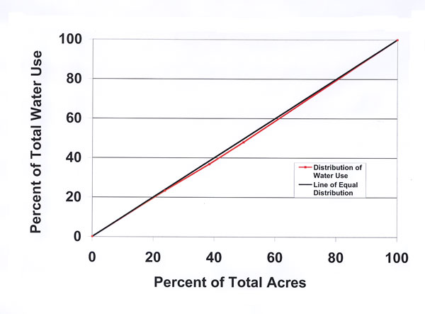
Figure 19. Distribution of total pecan water use relative to total pecan acres (2001, n = 340) (sorted by smallest to largest farm size group)
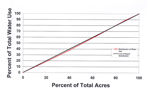
Figure 20. Distribution of total alfalfa water use relative to total alfalfa acres (2001, n = 524) (sorted by smallest to largest farm size group).
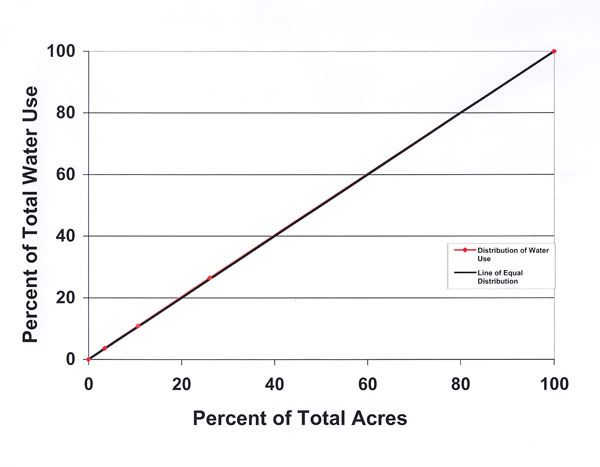
Figure 21. Distribution of total cotton water use relative to total cotton acres (2001, n = 164) (sorted by smallest to largest farm size group).
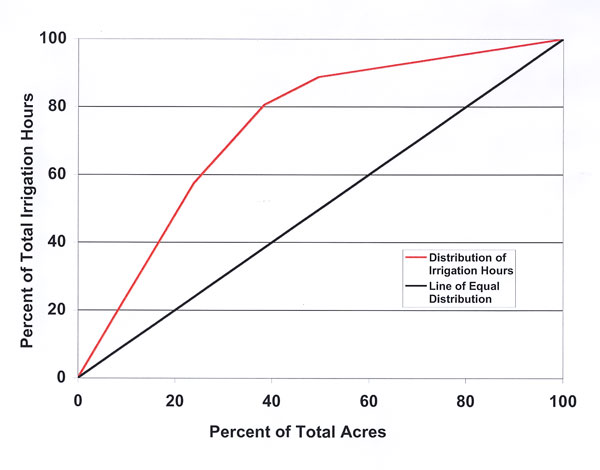
Figure 22. Distribution of total pecan irrigation hours relative to total pecan cres (2001, n = 340) (sorted by smallest to largest farm size group).
Figure 23. Distribution of total alfalfa irrigation hours relative to total alfalfa acres (2001, n = 524) (sorted by smallest to largest farm size group)
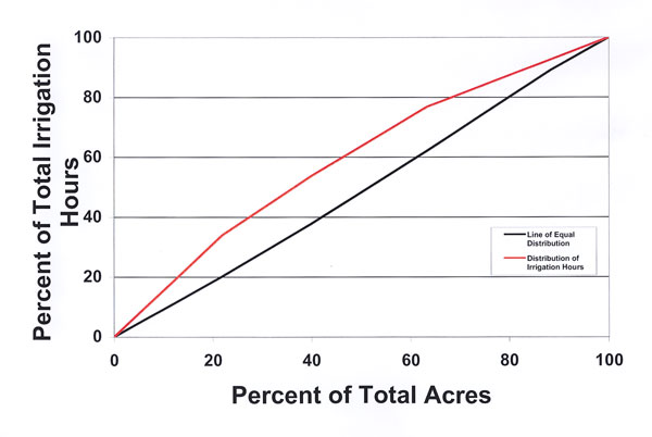
Figure 24. Distribution of total cotton irrigation hours relative to total cotton acres (2001, n =164) (sorted by smallest to largest farm size group).
Water Applied by Water Application Categories
The preceding research results have shown differences among irrigated parcels using a farm size stratification. Clearly, there are differences in total water applied for farms of different sizes. As stated above, the EBID water application data are based on engineering estimates, and numerous differences between recorded data and field measurements of water applied have been found. However, even with the limitations of the recorded data, the data can reveal large differences among irrigated parcels.
Figures 25, 26 and 27 show average acre-feet/acre/month of water applied for pecans, alfalfa and cotton for different levels of total 2001 irrigation season water use. In these figures, the top 10% of irrigated parcels received a greater amount of water than the remaining 90% of irrigated parcels; the top 25% received a greater amount of water than the remaining 75%, and so on. The fields were sorted from the highest to lowest annual total water applied. For pecans and cotton (figs. 25 and 26), the monthly totals applied by the different percentile groups are consistently ranked throughout the irrigation season. For cotton (fig. 27), there are some changes in monthly rankings at the beginning and end of the irrigation season, and the monthly totals are more tightly clustered than for either pecans or alfalfa.
Figures 25, 26 and 27 all include a reference line for maximum evapotranspiration over the growing season. For pecans (fig. 25), there appears to be equilibration or balancing between over-irrigation and under-irrigation across the months and between farm size groups. Alfalfa irrigation in excess of evapotranspiration (fig. 26) and deficit irrigation practices in cotton are again illustrated (fig. 27).
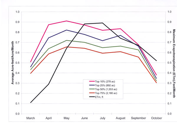
Figure 25. Average pecan acre-feet/acre/month by total pecan water application categories (2001, n = 340).
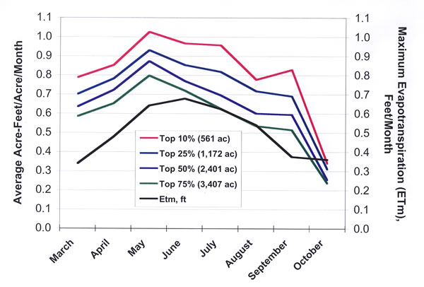
Figure 26. Average alfalfa acre-feet/acre/month by total alfalfa water application categories (2001, n = 524).
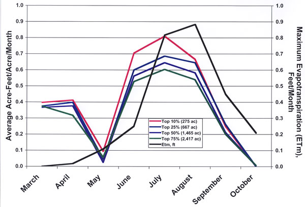
Figure 27 Average cotton acre-feet/acre/month by total cotton water application categories (2001, n = 164).
Irrigation Duration by Water Application Categories
Figures 28, 29 and 30 show average hours/acre/month for pecans, alfalfa and cotton for different levels of total water use. As above, the top 10% of irrigated parcels received a greater amount of water than the remaining 90% of irrigated parcels; the top 25% received a greater amount of water than the remaining 75%, and so on. The fields were sorted from the highest to lowest annual total water applied. Unlike the results shown above for total water applied by month, rankings of the different percentile groups are consistent throughout the irrigation season for pecans, alfalfa and cotton.
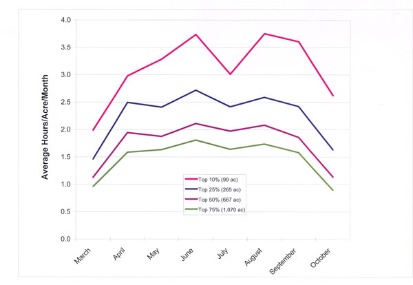
Figure 28. Average pecan hours/acre/month by total pecan water application categories (2001, n = 340).
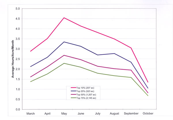
Figure 29. Average alfalfa hours/acre/month by total alfalfa water application categories (2001, n = 524).
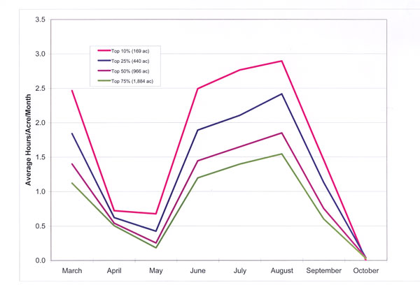
Figure 30. Average cotton hours/acre/month by total cotton water application categories (2001, n = 164
Conclusions and Implications
Based on this analysis of the irrigation district's 2001 water delivery records, approximately 16% (n = 54) of the 340 pecan farms analyzed applied water in excess of 5.0 acre-feet/acre, 52% (n = 273) of the 524 alfalfa farms analyzed applied water in excess of the 4.0 acre-feet/acre, and 40% (n = 66) of cotton farms applied in excess of 2.5 acre-feet/acre. These consumptive use benchmarks are based on the following yield assumptions and references: pecans, 5.0 acre-feet/acre for mature trees, yielding approximately 2,000 pounds per acre (Miyamoto, 1983); alfalfa, 4.0 acre-feet/acre for an established crop, yielding approximately seven tons per acre (Sammis, 1981; Simmons, 2003); cotton, 2.5 acre-feet/acre, yielding approximately 1,089 pounds/acre (Sammis, 1981). Many of the fields receiving water in excess of the consumptive use benchmarks are small, although excess applications also were received on larger-sized fields. Other parcels analyzed were found to be applying less than the consumptive use benchmarks.
Table 11 summarizes the data for fields which received water applications in excess of the consumptive use benchmarks discussed above. The total amounts of water applied in excess of consumptive use for the 54 pecan farms, 273 alfalfa farms, and 66 cotton farms were 298 acre-feet, 2,798 acre-feet, and 386 acre-feet, respectively. For pecans, 25.5% of the excess water was applied on farms of less than 5 acres, 18.8% applied on farms between 5 and 20 acres, and 55.7% on farms of greater than 20 acres. The distribution of excess water applied to alfalfa is less concentrated on the larger fields, with 39.5% of the excess applied to fields greater than 20 acres. Excess water applied to cotton is very biased to the larger fields, with 71.3% of the water applied to fields greater than 20 acres. These water distributions reflect the nature of the water delivery data received from the irrigation district.
Table 11. Total water applied in excess of consumptive use by farm size group, 2001.
| Total Water Applied in Excess of Consumptive Use | ||||||
| Pecans n = 54 |
Alfalfa n = 273 |
Cotton n = 66 |
||||
| Farm Size Group | Ac-ft | %Act-ft | Ac-ft | %Act-ft | Ac-ft | %Act-ft |
|
2 ≤ acres < 5 |
75.9 | 25.5 | 489.5 | 17.5 | 15.0 | 3.9 |
| 5 ≤ acres <10 | 29.4 | 9.9 | 439.0 | 15.7 | 29.1 | 7.5 |
| 10 ≤ acres < 20 | 26.6 | 8.9 | 765.1 | 27.3 | 66.5 | 17.3 |
| ≥ 20 acres | 165.9 | 55.7 | 1,104.3 | 39.5 | 275.0 | 71.3 |
| Total | 297.8 | 100.0 | 2,797.9 | 100.0 | 385.6 | 100.0 |
The research results presented here raise new questions and have many shortcomings. The results presented here demonstrate that there are differences in irrigation practices relative to farm size. However, the data used were not designed for analyzing irrigation practices relative to farm size. The primary objective of these data is for billing irrigators for water. Furthermore, the account observations obtained were not randomly selected from all EBID account holders or irrigators. Yet, the data proved to be a rich resource which had not been previously subjected to rigorous analysis. The results presented here should be interpreted carefully, and with the above shortcomings in mind.
Differences in farm size should be considered a proxy for a number of other characteristics of the irrigator population (for which data are currently unavailable), and it should be clear that the irrigator population is not homogeneous. As discussed above, irrigation duration may be a better indicator of water deliveries than the district-recorded data. And, interviews with irrigators lead to the conclusion that a portion of the irrigator population does not view long durations as problematic, and that dealing with the "problem" of long irrigation durations is very complicated (i.e., common property issues, easement disputes, etc.). Potential water savings from increased on-farm efficiency (through improved management, technology, or both) and irrigation infrastructure investments, or responses to incentives created by water marketing thus will vary by farm and throughout the irrigator population.
The loss of 46% of EBID's diverted water before deliveries to the farm turnouts is often cited by critics as an example of extreme inefficiency. However, the research described here has led to skepticism about the 54% diversion-to-delivery efficiency estimates. It is likely that at least part of the loss claimed to occur from diversion into EBID canals to delivery on farms is water applied to fields and not accounted for at the farm level. The district's water accounting procedures do not document this. It is also likely that carriage water requirements are larger for the smaller water deliveries to the smaller fields. Irrigation infrastructure on the smaller fields limits the rate at which water can be diverted to farms, resulting in deep percolation, runoff, and greater carriage water losses. Many necessary infrastructure improvements are unlikely to occur as a result of limited financial resources, easement disputes, disagreements between local irrigators, and lack of urgency or interest on the part of many irrigators.
Comparisons of EBID's estimates of water applied to derived estimates of water applied to the three crops (from yield functions and county average yields) raise more questions than can be currently answered. Additional research into on-farm irrigation efficiencies, harvest indices and water applied is needed in order to be confident about current measures of water applied to pecans, alfalfa and cotton in the Elephant Butte Irrigation District.
Field observations have led the authors to conclude that many water users appear to place a low priority on agricultural production. Yields for pecans in southern New Mexico vary greatly relative to orchard size, with orchards between two and five acres having an average yield of 636 pounds/acre while 1,754 pounds/acre is the average yield for orchards of at least 100 acres (U.S. Dept. of Agriculture, 1999). These yields were reported in the 1997 Census of Agriculture, and while members of the local pecan industry contacted in the course of this research do not dispute the range of yields between small and large orchards, they cite an average of ~850 pounds/acre for small orchards and at least 2,000 pounds/ acre in large, commercial, well-managed orchards. Reasons industry members give for low yields on small orchards include inadequate pruning, and limited fertility, pest and irrigation management. Similar variations in alfalfa and cotton management practices and yields are reported to exist; however, alfalfa and cotton are produced in several other regions in New Mexico, and census data for those two crops do not provide clear information about yield differences relative to farm size in the region encompassed by the Elephant Butte Irrigation District (where 75% of New Mexico's pecan production occurs).
Table 12 presents a summary of pecan orchard size distribution (using U.S. Census of Agriculture farm size classes), total irrigation water deliveries (for the 340 farms analyzed), average yields (from the 1997 Census of Agriculture), and average nut production per acre-foot of water delivered. The total amount of water recorded as delivered to these farms by EBID in the 2001 irrigation season was 11,022 acre-feet. The distribution of acres and acre-feet across farm sizes are remarkably similar, and again reflect the record-keeping assumption of approximately nine acre-inches per acre delivered by the district to the farm turnouts for the first irrigation of the season, and approximately six acre-inches for all subsequent irrigations. Multiplying average yields per acre (H) by total acres (D) gives total production by farm size class for the farms analyzed (I). Comparison of the distribution of farms (C) with distribution of production (J) across farm sizes illustrates the concentration of production on a small number of farms which characterizes New Mexico's overall pecan industry. Given the disparity in yields reported in the 1997 Census of Agriculture, nut production per acre-foot of water delivered (K) ranges from 161 pounds/acre-foot for the smallest orchards to almost 300 pounds/acre-foot for the largest orchards.
Table 12 results are based on EBID's accounting of how much water was delivered in a typical, full supply irrigation season (e.g., 2001). The findings of fieldwork in 2002 and 2003 lead to the tentative conclusion that nut production per acre-foot is probably less than presented in table 12 for the smaller orchards, and greater than the results in table 12 for the larger orchards. Column (K) is obviously not a measure of the marginal productivity or marginal value of water in pecan production, but it does provide insight into the physical efficiency of irrigation water used by pecan producers relative to orchard size.
| Farm size class1 | Farms2 | Farms % |
Acres2 | Acres % |
Acre-feet2 |
Acre-feet % |
Mean Yields per Acre (lbs)3 | Nut Production (tons) |
Production % |
Nut Production per Acre-foot (lbs) |
| (A) | (B) | (C) | (D) | (E) | (F) | (G) | (H) | (I) | (J) | (K) |
| 2–5 ac | 223 | 65.6 | 648 | 23.9 | 2,567.5 | 23.3 | 636 | 206.1 | 18.2 | 161 |
| 5–14.9 ac | 82 | 24.1 | 584 | 21.5 | 2,293.5 | 20.8 | 623 | 181.8 | 16.0 | 159 |
| 15–24.9 ac | 13 | 3.8 | 247 | 9.1 | 991.1 | 9.0 | 881 | 108.7 | 9.6 | 219 |
| 25–49.9 ac | 14 | 4.1 | 467 | 17.2 | 1,777.5 | 16.1 | 852 | 198.9 | 17.6 | 224 |
| 50–99.9 ac | 5 | 1.5 | 324 | 11.9 | 1,515.5 | 13.8 | 1,022 | 165.6 | 14.6 | 218 |
| 100–249.9 ac | 3 | 0.9 | 446 | 16.4 | 1,876.6 | 17.0 | 1,220 | 272.1 | 24.0 | 290 |
| Total | 340 | 100 | 2,716 | 100 | 11,021.7 | 100 | – | 1,133.2 | 100 | – |
|
1Farm size classes used in this table are those used in the 1997 Census of Agriculture for New Mexico pecan producers. |
||||||||||
It is commonly assumed by many observers and critics of EBID that the irrigation practices of the large, commercial farms must be improved in order to release water for other uses. However, the results of this and earlier research, the prevalence of deficit irrigation practices and other techniques or technologies currently used on large farms to increase the physical efficiency of irrigation water indicate that marginal increases in efficiencies on many large farms are likely to be small and come at a high cost. And the price at which many small-farm operators will be inclined to change their irrigation practices may be extremely high, because for them, irrigation appears to be a recreational, social, or lifestyle activity, rather than an income-generating pursuit. Furthermore, the common property nature of those segments of the water delivery system not owned by EBID creates a disincentive for investment and improvements by individual water users.
We currently hypothesize that many smaller EBID water users have minimization of the costs or risks of operating their small farms (regardless of the impacts on irrigation water productivity, yields, or total production) as their primary objective. Some smaller water users seem to have maximizing their utility or satisfaction from the small farm generally (and irrigation activities in particular) as a key objective. Again, these objective functions do not seem very compatible with the notion that water users generally will be interested in increasing irrigation efficiency through changes in technology, increases in management intensity, and responding to financial incentives to release surface water from agriculture for other competing uses.
The number of irrigated farms in the Elephant Butte Irrigation District has increased over the last several decades, due to splitting larger farms into smaller parcels. The ramifications of this for on-farm irrigation, delivery efficiencies, irrigation infrastructure, and irrigation system management are serious and underappreciated. One final conclusion of this research concerns the relationships between engineering and socio-economics. The conclusion is that the irrigation structures (e.g., physical items such as ditches, gates, turnouts, etc.) designed for the agricultural structure (i.e., the social organization of agriculture, reflected in the numbers and distribution of farms by size) which characterized the EBID in the early 20th century are currently a source of significant inefficiencies. The degree of reinvestment or disinvestments necessary to make irrigation structure compatible with current agricultural structure is surely very high. Furthermore, agricultural structure in Doña Ana County will continue to evolve with urbanization, population growth, and economic development. As a result, compatibility between irrigation infrastructure and agricultural structure is not a static target, given the dynamic nature of urban fringe agriculture in Doña Ana County.
References
Deras, J.R.D. 1999. Evaluation of Irrigation Efficiency and Nitrogen Leaching in Southern New Mexico. Unpublished master's thesis, New Mexico State University Department of Civil, Agricultural, and Geological Engineering, Las Cruces, N.M.
King, J.P. 2004. EBID Drought Update. Growers' meeting presentation, Las Cruces, N.M.
Magallanez, H. and Z. Samani. 2001. Design and Management of Irrigation Systems In Dry Climates. Paper presented at the FUNDAROBL International Conference, Caracas, Venezuela, July 2001.
Magallanez, H. 2003. Personal Communication. District Engineer, Elephant Butte Irrigation District, Las Cruces, N.M.
Miyamoto, S. 1983. Consumptive Water Use of Irrigated Pecans. Journal of the American Society of Horticultural Science 108(5):676-681.
Salameh Al-Jamal, M. T.W. Sammis and T. Jones. 1997. Nitrogen and Chloride Concentration in Deep Soil Cores Related to Fertilization. Agricultural Water Management 34(1):1-16.
Samani, Z. and N. Al-Katheeri. 2001. Evaluating Irrigation Efficiency in the Mesilla Valley. Paper presented to the American Society of Agricultural Engineers State Conference, Las Cruces, N.M.
Samani, Z., R. Skaggs, N. Al-Khatiri and J. Deras. 2004. Measuring On-Farm Irrigation Efficiency with Chloride Tracing Under Deficit Irrigation. Journal of Irrigation and Drainage Engineering, forthcoming.
Sammis, T.W. 1981. Yield of Alfalfa and Cotton as Influenced by Irrigation. Agronomy Journal 73:323-329.
Simmons, L. 2003. Crop Coefficients and ET for Pecans and Alfalfa in Las Cruces, NM. Unpublished research project paper, New Mexico State University, Dept. of Civil and Geological Engineering, Las Cruces, N.M.
Sinclair, T.R. 1998. Historical Changes in Harvest Index and Crop Nitrogen Accumulation. Crop Science 38(3):638-643.
U.S. Department of Agriculture. 1999. 1997 Census of Agriculture—New Mexico State and County Data. National Agricultural Statistics Service, AC97-A-31, Volume 1 Geographic Area Series, Part 31. Available online: http://www.nass.usda.gov/ .
U.S. Department of Commerce — Bureau of the Census. 1981. 1978 Census of Agriculture—New Mexico State and County Data. A78-A-31, Volume 1.
To find more resources for your business, home, or family, visit the College of Agricultural, Consumer and Environmental Sciences on the World Wide Web at aces.nmsu.edu
Contents of publications may be freely reproduced for educational purposes. All other rights reserved. For permission to use publications for other purposes, contact pubs@nmsu.edu or the authors listed on the publication.
New Mexico State University is an equal opportunity/affirmative action employer and educator. NMSU and the U.S. Department of Agriculture cooperating.
April 2005