Identification and Detection of Weeds on Irrigation Canals:
Survey of the Vegetation and Soils of the Leasburg Canal System, 2002-2006
RR-777
Jill Schroeder, Leigh Murray, April Ulery, Cheryl Fiore, Hien Nguyen and Xiaoli Liu
College of Agricultural, Consumer and Environmental Sciences, New Mexico State University
Authors: Respectively, Professor, Department of Entomology, Plant Pathology and Weed Science, New Mexico State University; Professor, Department of Statistics, Kansas State University; Professor, Department of Plant and Environmental Sciences, NMSU; Research Assistant, Department of Entomology, Plant Pathology and Weed Science, NMSU; Research Assistant, Department of Economics, NMSU; and Data Analysis Engineer, IM Flash Technologies, Lehi, UT.
Table of Contents
Executive Summary
Introduction
Materials and Methods
Results and Discussion
Relationship Between Canal and Soil Texture Categories
Numeric Soil Characteristics
Presence of Selected Vegetation Species as Affected by Canal Category or Soil Texture Category
Horsetail
Cyperus species
Bermudagrass
Rice cutgrass
Johnsongrass
Echinochloa species
Plantago species
Curly dock
Acknowledgments
References
Appendices
Executive Summary
The goal of this project was to characterize the vegetation and soils of the canals, laterals, and sublaterals of the Leasburg/Las Cruces/Mesilla canal system maintained by Elephant Butte Irrigation District (EBID). This work provides the first extensive database of canal and soil characteristics and vegetation during the peak of the irrigation season for the Leasburg system of the Elephant Butte Irrigation District (http://aces.nmsu.edu/academics/EPPWS/research-programs.html). The database included with this report will provide the basis for monitoring changes to the system over time, information from which to develop further research on the state of the canal system, and management strategies for the vegetation. Statistical models of vegetation presence will allow for prediction of future occurrence of important species and possible shifts in the vegetation community.
Since canal capacity is the most obvious characteristic of the system and because soil texture often influences vegetation presence, the data were analyzed first to examine the statistical relationship between canal capacity and soil texture and to compare canal capacities (or soil textures) with respect to soil characteristics, and then to model vegetation presence (i.e., the probability that a particular species or species category occurs at a particular location) where canal capacity (or soil texture) is the treatment factor and a soil characteristic is a covariate.
The canals within the Leasburg system were assigned to one of five capacity categories according to the EBID-recommended water-flow capacity, which ranged from 0.4 to 19.6 cubic meters per second (m3 s-1) (or 15 to 700 cubic feet per second [ft3 s-1]); canal category 1 was the largest and contained only the Leasburg Canal, while canal category 5 contained sublaterals with recommended flow rates of 0.4–0.8 m3 s-1 (15-29 ft3 s-1). A total of 236 sites, randomly located on these canals, laterals, and sublaterals, were surveyed once during each irrigation season between 2002 and 2006. Information obtained at each site included a digital photograph; Global Positioning System (GPS) coordinates; canal characteristics; a composite soil sample taken from the surface 12 cm and analyzed for the physical and chemical characteristics of soil texture, pH, electrical conductivity (EC), sodium adsorption ratio (SAR), organic matter (OM), nitrate-nitrogen (NO3-N), phosphorus (P), and potassium (K); and vegetation data, including percent of overall plant ground cover for each of the five dominant herbaceous plant species.
Soil characteristics varied widely along the canals, and did not necessarily reflect the properties of adjacent fields because canal soils may not be in situ but may have been moved around when the canals were constructed. Texture varied from sand to clay and was subsequently placed into coarse (sand, loamy sand), medium (sandy loam, sandy clay loam, silt, loam), and fine (sandy clay, clay, silty clay, clay loam, silty clay loam, silt loam) categories. Coarse-textured soils were more commonly found on the canals in categories 1 and 2, while fine-textured soils were more common on the smaller canals. Some extreme values of chemical characteristics, particularly EC and SAR, were observed; these were generally rare and may be related to the origin of the soil or human activities at these sites.
A total of 76 plant species or groups were identified; however, many plant species were present at only a few locations. Therefore, the 76 plant species or groups were further grouped into 13 species categories for statistical modeling. Of these 13 categories, the dominant species and genera identified on the canals included common bermudagrass (Cynodon dactylon), scouringrush or horsetail (Equisetum hyemale), rice cutgrass (Leersia oryzoides), Johnsongrass (Sorghum halepense), curly dock (Rumex crispus), Cyperus spp., Echinochloa spp., and Plantago spp. Presence of a vegetation group (i.e., the probability that a group occurred at a particular site) was modeled as a function of a treatment factor (either canal size or soil texture) and a soil characteristic by Analysis of Covariance models. If no soil characteristic was a significant predictor of presence, an Analysis of Variance model was fitted with either canal size or soil texture as the treatment factor.
Common bermudagrass, a creeping perennial grass, was the most common plant on the canals and was identified at 126 out of the 236 sampled locations (53.4%). Bermudagrass was more commonly found on the larger canals than on the smaller canals of this system. However, the soil characteristics potassium (K) and phosphorus (P) were found to be significant covariates for predicting bermudagrass presence on the canals. Bermudagrass was most likely to occur on the Leasburg Canal and on canals in category 2 regardless of the K or P concentration. However, bermudagrass was also predicted to be more commonly found on canals in the smallest category (canal 5) when K was low (minimum observed K = 20 mg kg-1) or P was high (maximum observed P = 62.5 mg kg-1).
When soil texture category was the treatment factor, bermudagrass was expected to occur at a probability greater than 0.4 regardless of soil texture or sodicity (represented by SAR), except for fine-textured soil at the minimum SAR = 0.74. As SAR increased above 13, probability of bermudagrass presence increased regardless of soil texture. Also regardless of soil texture, the probability of bermudagrass occurrence increased as either EC or P level increased.
Scouringrush (horsetail), a rhizomatous perennial related to ferns, was identified at 83, or 35.2%, of the locations surveyed. Horsetail was more likely to be found on the smaller, intermittent canals than the large continuous canals (categories 1 and 2). Specifically, horsetail presence was expected to be high on canals in categories 3 and 4 under non-saline conditions (minimum observed EC = 0.64 dS m-1 or SAR = 0.74) and over the entire range of EC or K values for canal category 5.
When soil texture was the treatment factor, horsetail presence generally decreased as the salinity (EC) or sodicity (SAR) increased for medium- and fine-textured soils. Horsetail presence decreased as K increased for fine-textured soils. In addition, horsetail presence was expected to be higher on soils with OM less than or equal to 1%, regardless of texture.
Rice cutgrass, a native creeping perennial grass, was identified at 39, or 16.5%, of the sampled locations. Rice cutgrass was predicted to be present more often (probability is greater than 0.5) on the Leasburg Canal (canal category 1) in sections where soil OM content was greater than 1.45%, regardless of texture, than on any other canal of the system. This species was not found on small canals (category 5) during this survey. When soil texture was the treatment factor, rice cutgrass tended to occur more frequently as SAR, K, or OM increased or as NO3-N decreased for all three texture categories.
Johnsongrass, a creeping perennial grass, was identified at 29, or 12.3%, of the locations. Johnsongrass was not found regularly on canals in any category, but analyses predicted that this species may be found most often on canals in category 3 on soils with high salinity (EC). When soil texture was the treatment factor, Johnsongrass would be predicted to occur most frequently on coarse-textured soil with pH of 7.25 (minimum observed pH) and least frequently on fine-textured soil.
Curly dock, a perennial broadleaf plant, was identified at 48, or 20.3%, of the locations. Three covariates, EC, SAR, and OM, were significant when canal category was the treatment factor; however, the results for salinity (EC) and sodicity (SAR) did not allow any consistent predictions for presence of this species to be made. However, as OM increased, curly dock occurred more frequently on the three smallest canal categories (3–5), while it occurred less frequently on the two larger canal categories (1 and 2). When soil texture was the treatment factor, as NO3-N increased, curly dock occurred more frequently in soils with coarse and medium texture but less frequently in soils with fine texture.
Cyperus species (C. esculentus and C. rotundus) are creeping perennial nutsedges and were identified at 58, or 24.5%, of the locations. Cyperus species had only one significant soil characteristic covariate, P, when either canal or soil texture was the treatment factor. As soil P increased, Cyperus species were predicted to occur more often on all canal categories or on all soil textures. However, these species were also most likely to be found on canals of category 3 and least likely to be found on canal category 1.
Echinochloa species (E. crus-galli and E. colona) are summer annual grasses and were identified at 67, or 28.4%, of the locations. None of the soil covariates affected presence of these plants on the canals; however, these species were predicted to occur most commonly on canals in category 4. The probability of finding these species was less than 0.4 in most cases when soil texture was the treatment factor, and, as P increased, the probability of Echinochloa species presence tended to decrease in soils with coarse and medium texture but to increase in fine-textured soil.
Plantago species (P. lanceolata and P. major), perennial broadleaf plants, were found at 82, or 34.7%, of the locations. Plantago species were relatively rare on canals in categories 1 and 5 and at locations with high salinity (EC) or sodicity (SAR). The probability of Plantago species presence was not affected by soil texture.
A wide variety of plants were found on the canals. Plant growth is desirable for erosion control and to provide valuable habitat for area wildlife. Therefore, management should perhaps be targeted to control specific species where they occur depending on
- The impact of the species on crops of the area and the species’ ability to transmit seeds into neighboring fields, which increases crop loss and the need for intensive weed management.
- The water used by individual plant species. Additional work under this project has evaluated water use by the plant species found to be most common on the canals relative to common bermudagrass under greenhouse conditions.
- The likelihood that plant growth will interfere with water flow in the canals. E.g., Equisetum (horsetail) poses a problem on the intermittent canals because the plant populations are increasing and occur in the bottom of the canals, disrupting water flow.
Introduction
Elephant Butte Irrigation District (EBID) maintains over 480 km of canals, laterals, and drains in southern New Mexico (EBID, 1998). This irrigation canal system of the middle Rio Grande basin is mainly a gravity-flow system. It contains and delivers irrigation water using compacted earthen canals and laterals within its boundaries, and includes rural and urban users. In general, the irrigation season runs from February to October each year (EBID, 1998). Irrigation water flows through two types of canals and laterals. One is the intermittent type that holds water only when someone is using the irrigation water from the canal or lateral. The other is the continuous type that holds water throughout the irrigation season.
A variety of vegetation is found along each of the different types of earthen canals, laterals, and drains. This vegetation may vary because of differences in soil characteristics, including soil texture, organic matter, salinity, and nutrient levels, as well as other canal and environmental factors. Many different and diverse plant species are seen on the canals and ditches in Doña Ana County, including the herbaceous weeds Johnsongrass (Sorghum halepense (L.) Pers.), Palmer amaranth (Amaranthus palmeri S. Wats.), yellow nutsedge (Cyperus esculentus L.), barnyardgrass (Echinochloa crus-galli (L.) Beauv.), junglerice (Echinochloa colona (L.) Link), Russian thistle (Salsola iberica Sennen), scouringrush or horsetail (Equisetum hyemale), common lambsquarters (Chenopodium album L.), common bermudagrass (Cynodon dactylon (L.) Pers.), and kochia (Kochia scoparia (L.) Schrad.). These weeds are widespread throughout the urban and rural areas of New Mexico and compete with desired vegetation for water and other valuable resources. Many of the weeds that grow along the canals may consume excessive quantities of water.
Mowing and the herbicide glyphosate are used by EBID to control the weeds along canals and roadways. However, herbicide use is generally limited to areas away from the canal due to liability concerns. In addition, certain weeds, such as horsetail, are not controlled by glyphosate. During the irrigation season, EBID mows each section of the canal system approximately every six weeks (EBID, personal communication), but some annual weeds can grow and produce seeds in less than six weeks (Aldrich and Kremer, 1997). Mowing often deposits the mature seeds into the canal system. Improvement of weed detection and management on irrigation canals is desired in order to improve irrigation efficiency and reduce weed movement into neighboring production fields and urban landscapes.
Current publications about the canal system of southern New Mexico do not include information about the soils and plants found on the canal banks. Therefore, the goal of this project was to characterize the vegetation and soils of the canals, laterals, and sublaterals of the canal system maintained by EBID.
Materials and Methods
General Site Description
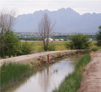
In this study, we targeted the Leasburg/Las Cruces/Mesilla canal system in southern New Mexico, which is maintained by the Elephant Butte Irrigation District (EBID). This system begins at the Leasburg Diversion Dam on the Rio Grande approximately 100 km north of El Paso, TX (U.S. Department of the Interior, Bureau of Reclamation [USDIBR], 2003). Located at the head of the Mesilla Valley, the Leasburg Diversion Dam is a concrete ogee weir with embankment wings that diverts water into the Leasburg Canal (USDIBR, 2003). The Leasburg Canal is 22 km long and has a recommended capacity of 19.6 cubic meters per second (m3 s-1) (or 700 cubic feet per second [ft3 s-1]) (USDIBR, 2003; EBID, 1998). It divides into two smaller canals and two large laterals (4.2–6.3 m3 s-1; 150–225 ft3 s-1), six medium laterals (1.7–2.5 m3 s-1; 60–90 ft3 s-1), 20 small laterals (0.8–1.4 m3 s-1; 30–50 ft3 s-1), and 22 sub-laterals (0.4–0.8 m3 s-1; 15–29 ft3 s-1) (Fiore et al., 2006; EBID, 1998). The Leasburg Canal carries irrigation water through the Mesilla Valley for the upper 12,800 hectares of the Mesilla Valley irrigation system (USDIBR, 2003). The Leasburg/Las Cruces/Mesilla canal system continues through the Mesilla Valley and ends south of the Mesilla Dam, which is on the Rio Grande 64 km north of El Paso (USDIBR, 2003). In total, the system is approximately 180 km long. A map is presented in Appendix A-1 to show the overall canal system surveyed in this research.
Selection of Locations for Sampling
An upper limit of 300 locations was initially chosen for sampling along the Leasburg/Las Cruces/Mesilla canal system. The number of locations was chosen to maximize sample size under logistical limitations of time and personnel. Locations were randomly distributed within the system proportionate to the distribution of major canals, laterals, and sublaterals to ensure an accurate representation of the system in the following way: The canals within the Leasburg system were assigned to one of five capacity categories according to the EBID-recommended water-flow capacity listed in Table 1. The canals and the category assignments are listed in Appendix A-2. Irrigation water in canals from categories 1 and 2 flows continuously during the irrigation season, while water in canals (laterals and sublaterals) from the remaining categories flows only when irrigation is requested by owners of water rights. For each canal category, the total length of canal was calculated and the proportion of the length was determined relative to the total length of the system (Table 1). Then the number of locations to be sampled within each canal category was decided by multiplying 300 locations by the category length proportion (Table 1). After that, for each canal category, the number of locations to be sampled for each segment (canal, lateral, or sublateral) within that category was determined by multiplying the number of locations on that category by the proportion of the segment length relative to the total length of the category. Because of calculation rounding, there were a total of 299 locations to be sampled, instead of 300, along the system. Finally, using a random number generator, 299 random numbers representing miles in tenths were obtained and randomly assigned to the list of segments (canals, laterals, and sublaterals) along the system according to the number of sample locations needed on the segment. The system map in Appendix A-1 shows the 299 randomly selected locations that were to be sampled along the Leasburg/Las Cruces/Mesilla canal system. Sampling locations were accessed by driving along the right side of the canal or lateral in the direction of the water flow to the selected point, assisted by GPS mileage readings.
Table 1. Recommended Canal Capacity, Length, Percent of Total Length, Planned Number of Sampled Locations, and Actual Number of Sampled Locations for Each Canal Category (total number of planned locations was 299; of that, 236 locations were sampled)
| Canal category |
Recommendeda capacity (m3 s-1) |
Lengthb (km) |
Percent of total |
Planned number of sample locations |
Actual number of sampled locations |
| 1c | 19.1 | 21.98 | 12.2 | 37 | 37 |
| 2d | 4.2–6.3 | 63.99 | 35.5 | 106 | 85 |
| 3e | 1.68–2.52 | 31.64 | 17.5 | 52 | 40 |
| 4f | 0.84–1.4 | 45.00 | 24.9 | 75 | 53 |
| 5g | 0.42–0.812 | 17.75 | 9.8 | 29 | 21 |
| aOriginal values were reported in ft3 s-1 (EBID, 1998). bOriginal values were reported in miles (EBID, 1998). cLeasburg Canal (EBID, 1998). dEBID category for Canal (EBID, 1998). eIntermediate category not addressed in EBID grouping (EBID, 1998). fEBID Lateral (EBID, 1998). gEBID Sublateral (EBID, 1998). |
|||||
Data Collection
Sampling only took place during the irrigation season once vegetation was fully established along the canals, generally mid June to late September, from 2002 to 2006. Appendix B shows monthly air temperatures and precipitation, as well as the irrigation and sampling periods for 2002 through 2006. At each location, data were collected using a 0.75 m by 1 m quadrat placed on the canal wall with the bottom of the quadrat at the water line. Data obtained at each location included a digital photograph, GPS coordinates (+/− 1 m accuracy), canal characteristics, spectral reflectance, a composite soil sample taken from the surface 12 cm, and vegetation data, including percent of overall plant ground cover for each of the five dominant herbaceous plant species. A total of 252 locations were sampled during the 2002 through 2006 irrigation seasons. The full data set is posted at http://aces.nmsu.edu/academics/EPPWS/research-programs.html.
The remaining 47 locations were not sampled due to either lack of access or the fact that the canal was lined with concrete. Five sampled locations were deleted from the final data set because of observed problems with vegetation being mowed or dead, and one sampled location was deleted because it was covered by seedling pecan trees. A further 11 sampled locations were deleted because soil analyses contained unreasonable or suspicious values. Therefore, 236 locations were analyzed for this project (Table 1).
Soil Analyses
A composite soil sample from each location was submitted to the New Mexico State University Soil, Water, and Agricultural Testing Lab to determine selected soil chemical properties and soil texture (Table 2; Gavlak et al. 2003). Soil characteristics varied widely along the canals, possibly because the soils may not be in situ but may have been disturbed or imported from other areas when the canals were constructed. Texture varied from sand to clay (note that no samples were classified as loam or silt) and was subsequently categorized into coarse (sand, loamy sand), medium (sandy loam, sandy clay loam, silt, loam), and fine (sandy clay, clay, silty clay, clay loam, silty clay loam, silt loam) textures. Observed ranges of soil variables, as well as biologically relevant values for each soil variable chosen from the literature (Herrera, 2000), are reported in Table 2.
Table 2. Selected Soil Parameters (analyzed by the Soil, Water, and Agricultural Testing Lab at NMSU, Las Cruces, NM) for the 236 Locations Sampled Through 2006 (methods are described in Gavlak et al. [2003])
| Test parameter | Range of observed results |
Biologically relevant values based on literaturea |
|
| Low | High | ||
| pH of saturation paste | 7.25–8.29 | 7.9 | 8.4 |
| Electrical conductivity (EC)b | 0.64 –39.90 dS m-1 | 4 | 16 |
| Sodium adsorption ratio (SAR)c | 0.74–43.12 | 13 | 30 |
| Organic matter (OM)d | 0.02–4.27% | 1 | 2 |
| NO3-Ne | 1.2–402.3 mg kg-1 | 10 | 30 |
| Phosphorus (P)f | 2.0–62.5 mg kg-1 | 7 | 23 |
| Potassium (K)g | 20–349 mg kg-1 | 30 | 60 |
| Texture of soil by feel | Sand–Clay; All textural classes except silt and loam were observed | ||
| aBased on nutrient or best management recommendations for local agronomic crops as reported in Herrera (2000). bElectrical conductivity of a saturation paste extract. cCalculated from the concentrations (mmol L-1) of Na, Ca, and Mg in a saturation paste extract, analyzed by inductively coupled plasma-optical emission spectroscopy. dOrganic matter, Walkley-Black method. e1:5 soil:water extract, cadmium reduction column. fNaHCO3 extractable, Olsen method. g1:5 soil:water extract, analyzed by inductively coupled plasma-optical emission spectroscopy. |
|||
Because we were concerned with vegetation growing along the irrigation canals in the Mesilla Valley (an important agricultural region in southern New Mexico), we chose to use biologically relevant values, in addition to low, high, and mean observed values, in statistical analyses of the soil properties and plant species distribution on the EBID canal system. The soil properties evaluated in this study are related to plant growth, and the upper and lower biologically relevant limits were selected based on agronomic definitions (Herrera, 2000). Adjustments to certain biological limits were made based on knowledge of area conditions and the fact that weeds tolerate a wide range of soil conditions (Ross and Lembi, 2009). In addition, many of these biologically limiting values are already used for definition purposes (e.g., EC ≥4 dS m-1 is defined as a “saline” soil) and in some cases as regulatory limits in other environments (e.g., NO3-N in water, although no soil NO3-N limits have been set).
Categories of Vegetation
Based on the final 236 sampled locations, a total of 76 plant species or groups were identified and are listed in Appendix C. Many plant species were present at only a few locations. Therefore, the 76 plant species or groups were further grouped into 13 species categories (Table 3) for statistical analysis. Table 3 also gives the number of sampled locations where each species or species category was one of the five dominant species at that location. The species categories included five individual species, three genera, and three family groups (Chenopodiaceae, Asteraceae, and Poaceae) (Table 3). The Poaceae were further grouped according to three life cycles: perennial, annual warm-season, and annual cool-season grasses.
Table 3. List of Species Within Each Category for Statistical Analysisa
| Species category | Common name(s) | Scientific name(s) | Number of locations (out of n = 236) where species category was one of the five dominant species categories |
| horsetail | scouringrush | Equisetum hyemale | 83 |
| Cyperus species | nutsedge species | Cyperus esculentus and C. rotundus | 58 |
| bermudagrass | bermudagrass | Cynodon dactylon | 126 |
| rice cutgrass | rice cutgrass | Leersia oryzoides | 39 |
| Johnsongrass | Johnsongrass | Sorghum halepense | 29 |
| perennial grasses | perennial grasses | Paspalum dilatatum, Leersia oryzoides, Sorghum halepense, Distichlis spicata, and Muhlenbergia asperifolia |
73 |
| Echinochloa species | barnyardgrass and junglerice | Echinochloa crus-galli and E. colona | 67 |
| warm-season annual grass species |
warm-season grasses | Cenchrus pauciflorus, Eriochloa gracilis, Leptochloa sp., Phalaris minor, Polypogon monspeliensis, Setaria lutescens, Chloris virgata, Leptochloa filiformis, Digitaria sanguinalis, Leptochloa uninervia, and Setaria verticillata |
52 |
| cool-season annual grass species |
cool-season grasses | Hordeum jubatum, Bromus spp., B. tectorum, and B. catharticus |
26 |
| Plantago species | plantain species | Plantago lanceolata, P. major, and Plantago spp. | 82 |
| curly dock | curly dock | Rumex crispus | 48 |
| Asteraceae species | aster species | Aster spinosus, Conyza canadensis, Helianthus ciliaris, Lygodesmia juncea, Sonchus oleraceus, Taraxacum officinale, Machaeranthera canescens, Baccharis glutinosa, and unidentified Asteraceae spp. |
98 |
| Chenopodiaceae species | common lambsquarters, kochia, and Russian thistle |
Chenopodium album, Kochia scoparia, and Salsola iberica | 24 |
| aThe complete list of species is given in Appendix C. | |||
Statistical Analyses
Since canal category is the most obvious characteristic of the system and because soil texture and chemistry often influence vegetation presence, the data were analyzed first to examine the statistical relationship between canal category and soil texture and to compare canal capacities (or soil textures) with respect to soil characteristics, and finally to model vegetation presence (i.e., the probability that a particular species or species category occurs at a particular location) where canal category (or soil texture) is the treatment factor and a soil characteristic is a covariate. Details of the statistical approach are provided here for future reference if additional analyses are conducted by readers of this report.
Chi-square test of homogeneity for canal category and soil texture. First, a chi-square (Χ2) test of homogeneity (Dowdy and Wearden, 1991) was performed at a significance level of α = 0.10 to compare canal category with respect to soil texture using the SAS FREQ procedure (SAS Institute, 2004). Prior to sampling, the number of locations to be sampled in each of the five canal categories was selected based on the proportion of the length of each canal to the overall length of all canals. However, the number of locations in each soil texture category was random (i.e., was determined only after the locations were actually sampled). Therefore, soil texture is the response variable and canal category is the treatment in this chi-square test. The parameters of interest for this chi-square test of homogeneity are πij, the probability of a location on canal i (i = 1,2,3,4,5) having soil texture j (j = 1,2,3), as given in the following display.
| Canal category | Soil texture | Total probability | ||
| Coarse | Medium | Fine | ||
| 1 | π11 | π12 | π13 | 1 |
| 2 | π21 | π22 | π23 | 1 |
| 3 | π31 | π32 | π33 | 1 |
| 4 | π41 | π42 | π43 | 1 |
| 5 | π51 | π52 | π53 | 1 |
For example, π32 is the true probability of a location on canal category 3 having a medium soil texture.
The null hypothesis is that the true proportion of locations with coarse (or medium or fine) soil texture is the same across the five canal categories. That is
Ho: π11= π21= π31= π41= π51
and π12= π22= π32= π42= π52
and π13= π23= π33= π43= π53
Analysis of Variance models to compare canal category (or soil textures) with respect to numeric soil characteristics. To determine if canal category differed with respect to means of numeric soil characteristics (e.g., pH; Table 2), we initially fitted analysis of variance (ANOVA) models using the SAS GLM procedure (SAS Institute, 2004) where each numeric soil characteristic was a response variable and canal category was the treatment factor. This analysis assumed that soil characteristics were normally distributed and had equal variances across canals. The null hypothesis was that canal category did not differ with respect to the average of each soil characteristic
Ho: μ1 = μ2 = μ3 = μ4 = μ5
where μi is the true mean soil characteristic for canal i. A similar analysis was performed with soil texture as the treatment factor, where i = 1,2,3 for coarse, medium, and fine texture instead of i = 1,2,3,4,5 for canal category. In addition, normality of residuals was checked using the Shapiro-Wilk test in the UNIVARIATE procedure (SAS Institute, 2004), and constant variance of residuals was checked using Levene’s test in the GLM procedure (SAS Institute, 2004). Problems with non-normality of residuals occurred for every soil characteristic except pH when either canal category or soil texture was the treatment factor. Non-normal residuals showed skewness toward higher values. In addition, problems with non-constant variance occurred for electrical conductivity (EC), sodium adsorption ratio (SAR), and organic matter (OM) when canal category was the treatment factor. These problems made the original ANOVA conclusions based on the normal distribution unreliable. Therefore, the ANOVA models were re-fitted using the technique of generalized linear models with the gamma distribution (appropriate for skewed data) and the log link function (McCullagh and Nelder, 1983) using the SAS GENMOD procedure (SAS Institute, 2004). A likelihood ratio (LR) chi-square test was used to test treatment differences. If the LR chi-square test for canal category or soil texture was significant at α = 0.10, pairwise comparisons were done using Wald chi-square tests (from the PDIFF option of the LSMEANS statement) to determine which treatments were different at a Bonferroni-adjusted significance level of α = 0.10/10 = 0.01 when canal category was the treatment factor and at α = 0.10/3 = 0.03 when soil texture was the treatment (the Bonferroni adjustment was done to control the Type 1 error rate). Note that when performing pairwise comparisons on treatment means, significant differences on the log scale imply similar significant differences on the data scale. In addition, confidence intervals on the data-scale means were also obtained, based on Wald Z-statistics (also from the LSMEANS statement), with a Bonferroni-adjusted confidence coefficient of 0.99 and 0.97 when canal category or soil texture was the treatment factor, respectively.
Logistic Analysis of Variance and Analysis of Covariance models to examine presence of vegetation species categories where canal category (or soil texture) is the treatment factor. For modeling vegetation presence (i.e., the probability that a particular species or species category occurs at a particular location), we examined logistic Analysis of Covariance (ANCOVA) models, another form of generalized linear model (Kutner et al., 2004; McCullagh and Nelder, 1983). Models with both canal category and soil texture factors were tried first to look at possible canal category and soil texture interactions. However, these models failed to converge, probably because of the low number of sampled locations in some canal category–soil texture combinations (see Table 1 and Results). Therefore, logistic ANOVA and ANCOVA models were fitted with canal category or soil texture as the single treatment factor. In ANCOVA models with canal category (or soil texture) as the treatment factor, one soil characteristic at a time was used as a covariate, while the response variable was the logit, defined as ln (π1ij / π0ij). For the case of canal category as treatment factor, the ANCOVA logistic model with unequal slopes (Kutner et al., 2004) is
ln (π1ij / π0ij) = β0i + β1i (xij) (1)
where i = 1,2,3,4,5, j = 1,2,3,…, ni = number of locations in canal i.
Here, ln (π1ij / π0ij) is the true logit (i.e., the natural log of the odds-ratio), π1iis the true probability that a particular species occurs at canal i and location j, π0ij is the true probability that the species does not occur at canal i and location j, β0i is the true y-intercept for canal i, β1i is the true slope for canal i, and xij is the observed value of the soil characteristic covariate measured at canal i and location j.
ANCOVA models are analogous to simultaneously fitting a regression line for each treatment (e.g., each canal category). Therefore, several hypotheses are of interest. First, is a common intercept appropriate for all canal categories? In terms of the parameters of the model, this null hypothesis is
Ho1: β01 = β02 = β03 = β04 = β05
Second, is the covariate slope equal to zero for all five canal categories? In terms of the parameters of the model, this null hypothesis is
Ho2: β11 = β12 = β13 = β14 = β15 = 0
If we fail to reject this null hypothesis, then the ANCOVA model is not appropriate and the ANOVA model is fitted instead (see below).
Third, if an ANCOVA model is appropriate, then the next hypothesis is: Is a common slope appropriate for all canal categories? That is, in terms of the parameters of the model, this null hypothesis is
Ho3: β11 = β12 = β13 = β14 = β15
If this common-slope null hypothesis is not rejected, then the ANCOVA model is refitted using one slope parameter, and the null hypothesis that the common slope, denoted as β1, is zero is tested
Ho4: β1 = 0
Fourth, if the ANCOVA model is appropriate, are the adjusted treatment means (i.e., the estimated mean response at the observed covariate mean ) the same for all canal categories? In terms of the parameters of the model, this null hypothesis is
![]()
where x..is the overall mean of the soil characteristic covariate. This test uses the usual adjusted treatment mean, which is the mean logit for a specific canal category at the mean observed value of the covariate. Other adjusted treatment means (i.e., at different values of the covariate) may be of interest. In this analysis, we also calculated adjusted treatment means for the minimum and maximum observed values of the covariate (β0i + β1i xmin and β0i + β1i xmax , respectively) and for low and high biologically relevant values chosen from literature.
The models are fitted on the logit scale, but the probability of presence or absence is naturally easier to understand. We can use the inverse link function to convert from the logit scale to the probability scale to get the probability of presence or of absence. The inverse link function in terms of the probability of presence is
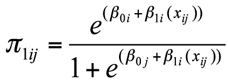
and therefore the probability of absence is
π0ij = 1 − π1ij
The relationship between the logit and the probability of presence is as follows: A negative logit corresponds to a probability that is less than 0.5, a logit of 0 corresponds to a probability of 0.5, and a positive logit corresponds to a probability of greater than 0.5.
Example graphs of the logistic ANCOVA models on the logit scale (Equation 1) for the case of two treatments are given in Figure 1 to illustrate the consequences of rejecting Ho1 and/or Ho3, assuming that Ho2 has been rejected (i.e., assuming the covariate is in the model for at least one treatment). If we fail to reject both Ho1 and Ho3, then there are both a common intercept and a common slope, and the two ANCOVA models reduce to the case of a single simple linear regression (Figure 1A). If we reject Ho1 and fail to reject Ho3, then there are different intercepts and a common slope, and the two ANCOVA models are analogous to the case of two simple linear regressions with different intercepts and a common slope (Figure 1B). If we fail to reject Ho1 and reject Ho3, then there are a common intercept and different slopes, and the two ANCOVA models are analogous to the case of two simple linear regressions with a common intercept and different slopes (Figure 1C). If we reject both Ho1 and Ho3, then there are both different intercepts and different slopes, and the two ANCOVA models are analogous to the case of two simple linear regressions with different intercepts and different slopes (Figure 1D). Also, in Figure 1, the three vertical lines crossing each simple linear regression line represent the locations of adjusted treatment means at the minimum (x_L), mean (x_bar), and maximum (x_H) observed values of the covariate, respectively. For example, in Figure 1D, for each simple linear regression line (or each treatment), the adjusted treatment mean increases when the observed value of the covariate increases from x_L to x_H. On the probability scale, this means that the probability of the presence of a particular species or species category increases when the soil characteristic (observed value of covariate) increases from x_L to x_H. Especially for the treatment that has a larger slope, the probability of presence increases quickly compared with the other treatment that has a smaller slope.
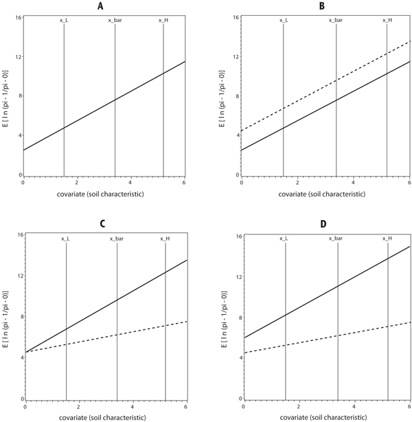
Figure 1. Graphs of Possible Analysis of Covariance models for two treatments for A. same intercept and same slope, B. different intercepts and same slope, C. same intercept and different slopes, and D. different intercepts and different slopes. Vertical axis is the expectation of the observed values on the logit scale defined as ln (π1ij / π0ij) = E[ln(pi_1/pi_0)] in Equation 1, and horizontal axis is soil characteristic (or observed value of covariate). The three vertical lines crossing each regression line represent (from left to right) locations of adjusted treatment means at x_L, x_bar, and x_H, respectively. x_L represents the minimum observed value of the covariate, x_bar represents the mean observed value of covariate, and x_H represents the maximum observed value of covariate.
The GENMOD procedure (SAS Institute, 2004) was used to fit logistic ANCOVA models with the binomial distribution and logit link function. Likelihood ratio (LR) chi-square statistics were used to test equality of intercepts (Ho1), all slopes equal to zero (Ho2), equality of slopes (Ho3), and equality of adjusted treatment means (“LSMEANS”) at the overall covariate mean (Ho5). When any of the chi-squares testing equality of parameters (i.e., Ho1, Ho3, and Ho5) were significant at α = 0.10, pairwise comparisons at the appropriate Bonferroni-adjusted significance level were performed using LR chi-square tests in CONTRAST statements. Note that when performing pairwise comparisons on adjusted treatment means, significant differences on the logit scale imply similar significant differences on the probability scale. In addition, maximum likelihood estimates were obtained for intercepts and slopes, and confidence intervals (with appropriate Bonferroni-adjusted confidence coefficients) were calculated for intercepts and slopes (LR-based confidence intervals [CIs] from the SOLUTION results) and for adjusted treatment means (“LSMEANS”) and other means at low and high values of the covariate (Wald-based CIs in ESTIMATE statements).
A common-slope ANCOVA was fitted when the LR test of equality of slopes, Ho3, was not rejected but the LR test that the common slope was equal to zero, Ho4, was rejected. An LR-based 90% confidence interval was calculated for the common slope, β1. Other inferences on non-slope parameters were conducted as for the unequal ANOVA models.
Overdispersion of ANCOVA logistic models was evaluated by Deviance and Pearson’s chi-squares and, in general, was not a problem.
If none of the soil characteristic covariates was significant for a particular vegetation category (i.e., the null hypothesis of all slopes equal to zero [Ho2] was never rejected), logistic ANOVA models were fitted where canal category (or soil texture) was the treatment factor and the response variable was the logit, again defined as ln (π1ij / π0ij). For canal category as treatment factor, the model is
ln (π1ij / π0ij) = μi (2)
where i = 1,2,3,4,5, j = 1,2,3,…, and ni = number of locations in canal i.
Here, π1ij, π0ij, and ln (π1ij / π0ij) are defined the same as in the previous ANCOVA model, and μi is the mean for canal i. The hypothesis of interest is equality of the treatment means
Ho6: μ1 = μ2 = μ3 = μ4 = μ5
The inverse link function in terms of the probability of presence is
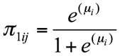
and therefore the probability of absence is
π0ij = 1 − π1ij
Figure 2 shows the situation for ANOVA models on the logit scale (Equation 2) for the case of two treatments. In Figure 2, the null hypothesis of all slopes equal to zero (Ho2) was not rejected. That tells us that there was no covariate in the model (or slopes are zero) for all treatments. Therefore, there are only horizontal lines in Figure 2. If we fail to reject Ho6, then there is a common intercept, and all the treatments have the same horizontal-line model (Figure 2A). If we reject Ho6, then there are different intercepts, and at least one treatment has a different ANOVA model from other treatments (Figure 2B). Also, in Figure 2, analogous to ANCOVA models in Figure 1, the vertical lines crossing each horizontal line represent the locations of treatment means at the minimum (x_L), mean (x_bar), and maximum (x_H) observed soil characteristic values, respectively. Note that in Figure 2B, for each horizontal line (each treatment), the treatment mean does not change when the soil characteristic value increases from x_L to x_H (unlike the ANCOVA models in Figure 1). On the probability scale, this means that the probability of a particular species or species category being present is the same over the range of soil characteristic values (from x_L to x_H ).
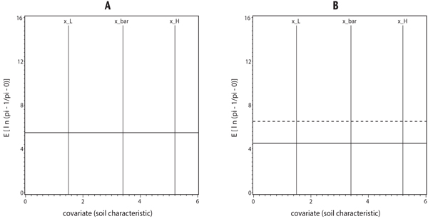
Figure 2. Graphs of Possible Analysis of Variance models for two treatments for A. same intercept and B. different intercepts. Vertical axis is the expectation of the observed values on the logit scale defined as ln (π1ij / π0ij) = E[ln(pi_1/pi_0)] in Equation 2, and horizontal axis is soil characteristic. Vertical lines across each horizontal line represent (from left to right) locations of treatment means at x_L, x_bar, and x_H, respectively. x_L represents the minimum observed value of soil characteristic, x_bar represents the mean observed value of soil characteristic, and x_H represents the maximum observed value of soil characteristic.
The logistic ANOVA models were also fitted using the GENMOD procedure (SAS Institute, 2004) with binomial distribution and logit link function and with treatment factor being either canal category or soil texture. Tests and confidence intervals were performed similar to analyses of the gamma ANOVA models with soil characteristics as responses, except that all tests and confidence intervals in the logistic ANOVA models were based on LR techniques. Given the number of locations in this study, differences between LR and Wald techniques were negligible. Overdispersion of ANOVA logistic models was again evaluated by Deviance and Pearson’s chi-squares.
We note one caveat when interpreting a significant test (i.e., rejecting Ho1, Ho3, Ho5, or Ho6) and subsequent pairwise comparisons and confidence intervals. As described previously, overall tests are rejected at α = 0.10, and subsequent comparisons are tested at a Bonferroni-adjusted level of α/k, where k is the number of pairwise comparisons. Bonferroni confidence intervals on parameters are likewise calculated at a confidence coefficient of 1 − α/k. In some cases, because of their conservative nature, the Bonferroni pairwise comparisons and confidence intervals give results that conflict with the overall test results. In these cases, the results of the overall test will be used for interpretation. Such cases will be noted in the results.
Results and Discussion
Relationship Between Canal and Soil Texture Categories
Soil characteristics varied widely along the canals, and did not necessarily reflect the properties of adjacent fields because canal soils may not be in situ but may have been moved around when the canals were constructed, as seen in Appendix A-3. The counts of soil texture for each canal category are listed in Table 4. The chi-square test of homogeneity, which was performed to compare canal capacity categories with respect to occurrence of soil texture, gave a chi-square value of Χ2(8) = 65.67, with p < 0.0001. At α = 0.10, we rejected the null hypothesis that the probability of sampling coarse (or medium or fine) soil texture is the same across the five canal categories. Therefore, we conclude that the proportion of locations with coarse (or medium or fine) soil texture was not necessarily the same across the five canal categories. Examination of observed counts versus expected counts (Table 4) shows that, for coarse texture, observed counts were greater than expected counts in the largest capacity canals (categories 1, 2, and 3) and lower than expected counts in canals from categories 4 and 5. An opposite pattern was seen for fine texture. Medium texture did not show a strong pattern across canals.
Table 4. Canal by Soil Texture Category Chi-Square Test of Homogeneity. Χ2 (df = 8) = 65.6679, p < 0.0001.
| Soil texture category; Observed counta [top], expected count [middle], observed row percent [bottom] |
||||
| Canal category |
Coarse | Medium | Fine | Row-total observed count |
| 1 | 17 11.29 45.95 |
14 15.21 37.84 |
6 10.50 16.22 |
37 |
| 2 | 34 25.93 40.00 |
41 34.94 48.24 |
10 24.13 11.76 |
85 |
| 3 | 14 12.20 35.00 |
21 16.44 52.50 |
5 11.36 12.50 |
40 |
| 4 | 5 16.17 9.43 |
14 21.78 26.42 |
34 15.05 64.15 |
53 |
| 5 | 2 6.41 9.52 |
7 8.63 33.33 |
12 5.96 57.14 |
21 |
| Column-total observed count |
72 | 97 | 67 | 236 |
| a“Observed count” is the number of sites observed in each canal category by texture category. “Expected count” is the expected number of sites in each canal category by texture category under the null hypothesis of no difference between canals in occurrence of soil textures. “Observed row percent” is the percent of sites in each soil texture for a canal category. Row percents add to 100% within each row. | ||||
As noted previously, there were small observed counts in some cells (Table 4), which is not surprising given that the sampled number of locations on canals of different capacities was proportional to the length of canals in that capacity, and we had no a priori knowledge of what soil textures to expect. From a statistical standpoint, the chi-square test of homogeneity is an approximate test that may be unreliable if the number of cells with expected counts is 5 or less. In this case, expected counts for all canal category–soil texture combinations are above 5, implying that these results are reliable.
Numeric Soil Characteristics
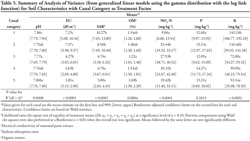
Canal as treatment factor. Results are summarized in Table 5 for analysis of variance models to compare canals with respect to the numeric soil characteristics pH, EC, SAR, OM, NO3-N, P, and K (Table 2). From the p-values of the treatment chi-squared tests, canal categories did not differ with respect to mean P at α = 0.10. However, the null hypothesis was rejected for all other characteristics. Specifically, for EC, SAR, and K, pairwise comparisons show that the highest capacity canals (categories 1 and 2) were statistically not different and had high means. In comparison, canals in categories 3, 4, and 5 were statistically not different from each other, but had lower means than canals in categories 1 and 2. Pairwise comparisons show that canals in categories 1 and 5 had similar high mean pH, while canals in categories 2, 3, and 4 had lower mean pH. For OM, only canals in category 3 (low OM) and 5 (high OM) were different. For NO3-N, canal 1 was statistically lower than the other four, which were not different.
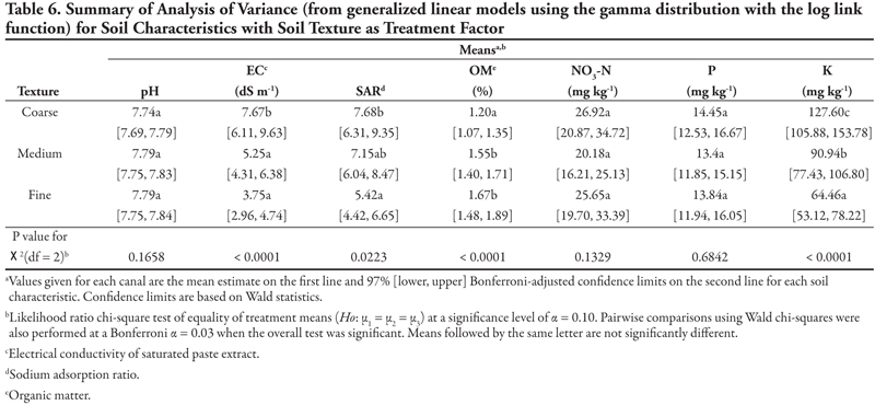
Soil texture as treatment factor. Results are summarized in Table 6 for analysis of variance models to compare soil texture with respect to numeric soil characteristics. From the p-values of the chi-squared tests, soil texture categories did not differ with respect to mean pH, NO3-N, or P. In comparison, the null hypothesis was rejected for EC, SAR, OM, and K. In particular, pairwise comparisons indicate that while coarse texture differed from medium and fine textures in having higher mean EC and lower mean OM, medium and fine textures were not different. For mean K, coarse, medium, and fine textures were all different from each other, with a gradient of coarse (highest mean K) through medium to fine (lowest mean K). For SAR, coarse (high SAR) and fine (low SAR) textures were different from each other but not from medium texture.
Interpretation of these soil results is difficult because samples at each location represent a single point in time and space. The results provide information to be used as the basis for further study of the differences in soil properties as influenced by canal capacity or other canal characteristics. Except for the unusually high values that may have been caused by isolated incidents, most of the values measured for the standard soil analyses were within the expected agronomic range; for example, the pH was near neutral to slightly alkaline at most sites, as would be expected in a semi-arid, irrigated region. Even though there were significant differences in pH relative to canal capacity, the differences were not sizable enough to matter biologically to most plant species. As we gain more information and understanding about the weed species found in this system, we may be able to use this statistical relationship to identify a potential feature that supports or inhibits weed growth along the canals.
When one soil property was extremely high, it was not surprising to find that several other properties were also very high, since soil properties are often co-dependent. For example, EC reflects contributions from all soluble ions including sodium (which affects SAR), NO3-N, and K. This information helped us identify locations of concern. In general, one would not expect high nutrient levels (NO3-N, P, K) or organic matter (OM) along the canals because these have been in place for many decades and have not been supplemented with agricultural amendments. One of the more surprising results was the lower EC observed on the smaller capacity canals (Table 5). The smaller canals often have intermittent water flow, which could lead to periods of evaporation and deposition of salts at the soil surface. Perhaps the intermittent water flow also flushed out any accumulated salts and thus lowered the EC along these smaller canals. While such speculation is interesting, it is not proven by the data presented in this report. In fact, the purpose of this report is to alert investigators to possible relationships in the hope that more detailed and comprehensive studies can be done to establish and explain the true causes of results reported herein.
Presence of Selected Vegetation Species as Affected by Canal Category or Soil Texture Category
In the following section, we discuss Analysis of Covariance (ANCOVA) models for the following eight species and genera combinations: horsetail, Cyperus species, bermudagrass, rice cutgrass, Johnsongrass, Echinochloa species, Plantago species, and curly dock (Table 3). Bermudagrass was the most commonly found species in the survey (Table 3) and was identified at 126 out of the 236 sampled locations (53.4%). Horsetail was identified at 83 (35.2%) locations, while rice cutgrass, Johnsongrass, and curly dock were identified at 39 (16.5%), 29 (12.3%), and 48 (20.3%) locations, respectively. Categories for the genera Cyperus, Echinochloa, and Plantago each contained two species and were identified at 58 (25%), 67 (28%), and 82 (35%) locations, respectively.
The family categories (Asteraceae and Chenopodiaceae), warm-season annual grasses, cool-season annual grasses, and perennial grasses (Table 3) will not be discussed here for the following reasons. The Asteraceae and warm-season annual grasses categories each included more than 8 species. As a whole, these two groups were large, and results lack meaning because of the diversity of species included in these categories and because each species was represented by only a few locations (Table 3 and Appendix C). The Chenopodiaceae and cool-season annual grasses categories included too few locations to analyze reliably. The perennial grasses category included rice cutgrass and Johnsongrass, which made up the majority of the locations and were analyzed separately. The results for the remaining species categories are summarized in Appendix D.
Results are presented in table form to provide complete information about the fitted models and values of the covariates, and so that graphs can be constructed by the reader as desired. In discussing results of the ANCOVA model for a species or genera category, we first discuss the tests of intercepts and slopes, referring back to the null hypotheses and figures in the Materials and Methods section. We then summarize where the ANCOVA model predicts that plant type to occur with relatively high probability of occurrence of 0.40 or higher. Finally, we summarize the information in light of what is known about the life cycle and habitat characteristics of each species or genera. Tables summarizing ANCOVA (or ANOVA) results are placed at the end of each species or genera section.
Horsetail
Horsetail is a primitive, native, creeping perennial that reproduces vegetatively by an extensive system of underground rhizomes and by spores (DiTomaso and Healy, 2007). The habitat where horsetail is reported to commonly occur is moist, sandy, marshy areas, including riparian areas and ditches. As discussed in detail in the following sections, the plant was most commonly found on the smaller, intermittent canals and laterals (especially in non-saline soil), and was rare on the largest canal (Leasburg canal), possibly because of the continual water flow. The analyses suggest that horsetail is predicted to more likely be present on fine-textured soils than coarse soils. This result is not supported by the limited available literature, however, suggesting that additional work is needed to further assess the relationship between horsetail invasion and soil texture and chemistry. Horsetail presence was not influenced by soil pH, OM, NO3-N, or P in this survey.
Canal category as treatment factor: Horsetail had three significant soil characteristic covariates (EC, SAR, and K), the effects of which were not consistent over canal categories, resulting in logistic ANCOVA models with unequal slopes (Tables 7, 8, and 9, respectively). We discuss Table 7 in detail, referring back to the first four null hypotheses and Figure 1 from the Materials and Methods section. The remaining tables summarizing unequal slopes in ANCOVA models are interpreted similarly to Table 7.
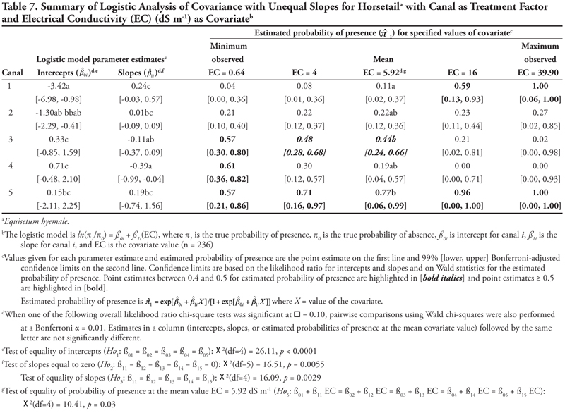
First, the null hypothesis of equal intercepts (Ho1) was rejected (p < 0.0001), indicating different probability of horsetail presence if EC = 0 (as in Figure 1B or 1D). Specifically, canal categories 1 and 2 (the largest canals) had significantly negative intercepts (on the logit scale), indicating a low (![]() < 0.2) probability of occurrence if EC = 0. In comparison, intercepts for canal categories 3, 4, and 5 were not significantly different from zero (on the logit scale), as evidenced by the 99% confidence intervals, which contained zero. This indicates a probability of horsetail presence of approximately
< 0.2) probability of occurrence if EC = 0. In comparison, intercepts for canal categories 3, 4, and 5 were not significantly different from zero (on the logit scale), as evidenced by the 99% confidence intervals, which contained zero. This indicates a probability of horsetail presence of approximately ![]() = 0.5 on canals in categories 3, 4, and 5. Thus, the plant was more likely to be found on the smaller, intermittent canals than the large continuous canals (categories 1 and 2) if EC = 0. (Note that the y-intercept is just the predicted probability of presence if EC = 0. This does not imply that zero is a reasonable value for EC or any other covariate. Rather, the different intercepts in the ANCOVA model imply that an individual model for one canal category [or soil texture] is at a higher or lower level than another canal category’s model [see Figure 1B and 1D]. A y-intercept is typically included in regression models for better fit of the data, even if β0 = 0 is physically unreasonable.)
= 0.5 on canals in categories 3, 4, and 5. Thus, the plant was more likely to be found on the smaller, intermittent canals than the large continuous canals (categories 1 and 2) if EC = 0. (Note that the y-intercept is just the predicted probability of presence if EC = 0. This does not imply that zero is a reasonable value for EC or any other covariate. Rather, the different intercepts in the ANCOVA model imply that an individual model for one canal category [or soil texture] is at a higher or lower level than another canal category’s model [see Figure 1B and 1D]. A y-intercept is typically included in regression models for better fit of the data, even if β0 = 0 is physically unreasonable.)
Second, the null hypothesis of slopes equal to zero (Ho2) was also rejected (p = 0.0055), indicating that an ANCOVA model (as opposed to an ANOVA model) was appropriate. Next, the null hypothesis of equal slope (Ho3) was rejected (p = 0.0029), indicating that the relationship between probability of horsetail presence and EC was not the same over the five canal categories (as in Figure 1D). Specifically, the slope for canal category 4 was significantly negative, while all remaining slopes were not different from zero (as in Figure 2B), as evidenced by the conservative 99% confidence intervals.
These fitted ANCOVA models lead to the following general conclusions about horsetail presence at different levels of the covariate EC on different canal capacity categories. Horsetail presence was expected to be high (>0.5) in non-saline soils (minimum observed EC = 0.64 dS m-1) on the small canals (categories 3, 4, and 5) and over the entire range of EC values for canal 5 (Table 7). Horsetail was also predicted to occur with high probability on canal 1 (Leasburg) at high EC ≥ 16; however, this is an unlikely situation given the fact that few samples had extremely high EC (Table 5), and resulting confidence intervals were very wide (Table 7).
Finally, the null hypothesis of equal mean response at the mean observed EC value of 5.92 dS m-1 (Ho5) was rejected (p = 0.0340), indicating that the probability of horsetail being present differed among the five canal categories at the mean EC. Specifically, at mean EC (5.92 dS m-1), the highest probability of horsetail presence ( ![]() = 0.77) was on canals in category 5, while the lowest probability (
= 0.77) was on canals in category 5, while the lowest probability ( ![]() = 0.11) was on canal category 1.
= 0.11) was on canal category 1.
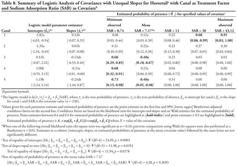
A very similar pattern is seen in Table 8 for SAR as the covariate with respect to intercepts and slopes. Horsetail presence was expected to be high on canals in categories 3, 4, and 5 for the minimum observed SAR (0.74) and on canal category 1 at extreme values of SAR (>30). However, the prediction of horsetail presence at these high values of SAR is unreliable, as evidenced by very wide confidence intervals, because of few observations. At the mean observed SAR of 7.17, however, predicted probability of horsetail presence was not different among five canal categories.
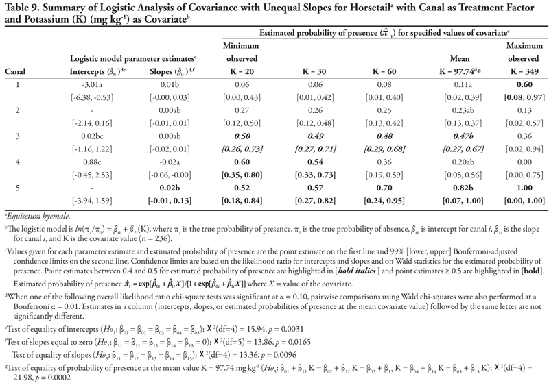
A similar pattern is seen in Table 9 for K as the covariate. Here, only canal category 1 had a significant (negative) intercept, while the slope was again significantly negative for canal category 4 and not significantly different from zero for canals in categories 1, 2, 3, and 5. Overall, horsetail presence was predicted to be high ( ![]() > 0.52) on canals of category 5 regardless of the level of K, and on canal categories 3 and 4 at K ≤ 60 mg kg-1, similar to what was observed for the covariates EC and SAR. At the mean observed K (97.74 mg kg-1), probability of horsetail presence decreased with increasing canal size category, similar to EC.
> 0.52) on canals of category 5 regardless of the level of K, and on canal categories 3 and 4 at K ≤ 60 mg kg-1, similar to what was observed for the covariates EC and SAR. At the mean observed K (97.74 mg kg-1), probability of horsetail presence decreased with increasing canal size category, similar to EC.
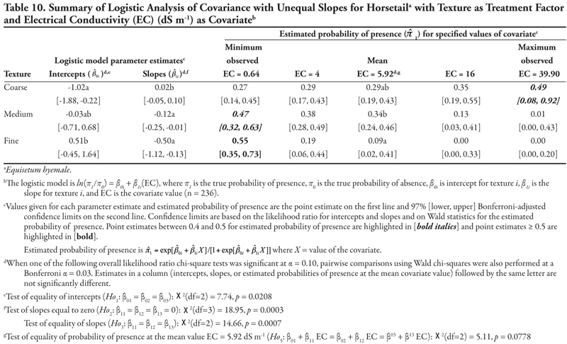
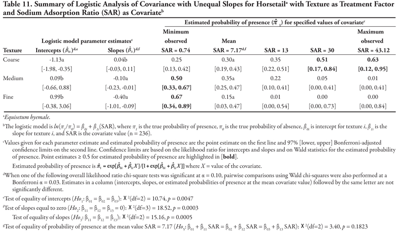
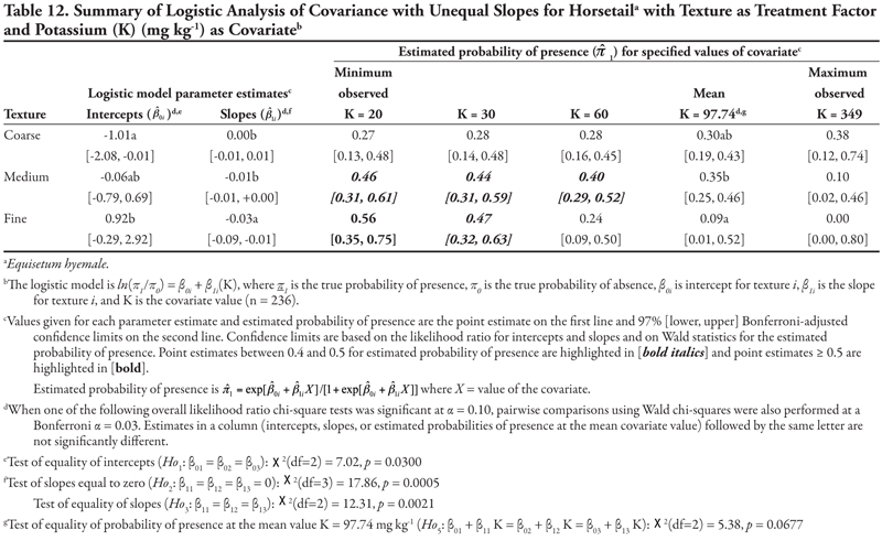
Soil texture as treatment factor: Horsetail had the same three significant soil characteristic covariates with unequal slopes (EC, SAR, and K; Tables 10, 11, and 12, respectively; Figure 1D) and one additional covariate with equal slope (OM, Table 13). For EC and SAR ANCOVAs, only the intercept for coarse soil texture was significantly different from zero (negative), while slopes for both medium and fine soil textures were significantly negative and not different from each other (Tables 10 and 11, respectively). With regard to predicted probability of horsetail presence, horsetail was more likely to occur in fine-textured soils at the minimum observed EC of 0.64 dS m-1 (![]() = 0.55), or in fine and medium soil textures at minimum observed SAR of 0.74 (
= 0.55), or in fine and medium soil textures at minimum observed SAR of 0.74 (![]() > 0.50). Horsetail presence generally decreased as the covariate levels increased, except for coarse-textured soils at high SAR (≥ 30), although the prediction is unreliable because of few observations (Tables 5 and 11). A similar pattern was observed for K (Table 12) except that the slope was only significantly different from zero for fine soil texture. Horsetail had the highest predicted probability of occurrence for fine-textured soils at the minimum observed K of 20.00 mg kg-1.
> 0.50). Horsetail presence generally decreased as the covariate levels increased, except for coarse-textured soils at high SAR (≥ 30), although the prediction is unreliable because of few observations (Tables 5 and 11). A similar pattern was observed for K (Table 12) except that the slope was only significantly different from zero for fine soil texture. Horsetail had the highest predicted probability of occurrence for fine-textured soils at the minimum observed K of 20.00 mg kg-1.
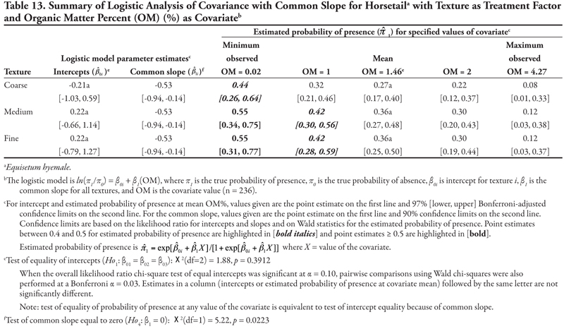
When OM was evaluated as a covariate, the null hypothesis to test common slope (Ho3) was not rejected, and hence the ANCOVA model with common slope was fitted and Ho1 and Ho4 were tested (Table 13). Such an ANCOVA model results in parallel lines (as in Figure 1B) if intercepts are statistically different from each other (i.e., Ho1 is rejected), or a single model (as in Figure 1A) if intercepts are not statistically different (i.e., Ho1 is not rejected). In this case, intercepts were not statistically different from each other (p =0.3912) and the common slope was significantly negative (p = 0.0223), resulting in a plot like Figure 1A but with a line that decreases from left to right. Overall, horsetail was predicted to be present with a high probability when OM was < 1% in medium- and fine-textured soils ( ![]() = 0.55) and with a moderate probability (
= 0.55) and with a moderate probability (![]() = 0.44) when OM was 0.02% on coarse-textured soils or when OM was 1% on medium- and fine-textured soils (
= 0.44) when OM was 0.02% on coarse-textured soils or when OM was 1% on medium- and fine-textured soils (![]() = 0.42).
= 0.42).
Cyperus species
Cyperus species are creeping perennial weeds of worldwide distribution that reproduce vegetatively by tubers, are commonly found in disturbed agricultural areas (including irrigation ditches), and tolerate a wide range of soil conditions (DiTomaso and Healy, 2007). The following results suggest that these species become more common as P concentrations increase on all canals and textures. Other soil characteristics, such as salinity, sodicity, organic matter, K concentration, or pH, have little influence on Cyperus spp. presence on these canals.
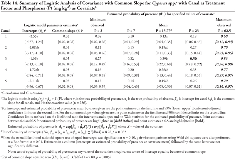
Canal category as treatment factor: Cyperus species (C. esculentus and C. rotundus) had only one significant soil characteristic covariate—phosphorus (P)—the effects of which were consistent over canal categories, resulting in logistic ANCOVA models with a common positive slope (Table 14, Figure 1B). Intercepts were statistically different but were all negative, indicating low probability of presence if P = 0. If P = 0, Cyperus spp. would most likely occur on canals in category 3 (estimated logit = −1.09, ![]() = 0.25) and least likely occur on canal category 1 (estimated logit = −2.55,
= 0.25) and least likely occur on canal category 1 (estimated logit = −2.55, ![]() = 0.07). Overall, Cyperus spp. are predicted to occur most frequently on canals in category 3, regardless of P level; however, probability of occurrence was ≥ 0.39 when P levels were 13.77 mg kg-1 (mean observed) or greater. Probability of observing Cyperus spp. was high on all canals when P was at the maximum observed value of 62.5 mg kg-1, but these latter probability estimates are unreliable (as evidenced by the wide 99% confidence intervals) due to small sample size.
= 0.07). Overall, Cyperus spp. are predicted to occur most frequently on canals in category 3, regardless of P level; however, probability of occurrence was ≥ 0.39 when P levels were 13.77 mg kg-1 (mean observed) or greater. Probability of observing Cyperus spp. was high on all canals when P was at the maximum observed value of 62.5 mg kg-1, but these latter probability estimates are unreliable (as evidenced by the wide 99% confidence intervals) due to small sample size.
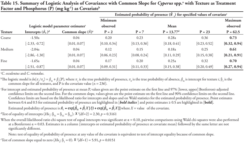
Soil texture as treatment factor: When soil texture was the treatment factor, Cyperus spp. again had only P as a significant covariate, with a common positive slope (Table 15, Figure 1A). Intercepts were not statistically different from each other (p = 0.3161) but were negative, indicating that if P = 0, Cyperus spp. had a similar low probability of occurrence for all three soil texture categories. The probability of finding Cyperus spp. on all soil textures increased consistently as P concentration increased. This pattern was very similar to that observed when canal was the treatment factor.
Bermudagrass
Bermudagrass is a warm-season creeping perennial grass that reproduces by means of an extensive system of creeping rhizomes and stolons and by seed (DiTomaso and Healy, 2007). The habitat for this species includes most disturbed sites that receive some warm-season moisture. The plant tolerates a wide range of pH conditions and saline soils. The following results suggest that bermudagrass is one of the most commonly found species on the irrigation canals; is found more often on large, continuous flow canals, regardless of soil texture; and can tolerate high P, low K, and high salinity or sodicity. Soil pH or NO3-N concentration had no effect on bermudagrass presence in this survey. These results are consistent with what is known about the species. Bermudagrass has been suggested as a species that may provide canal bank stability; however, a related study suggested a relationship between bermudagrass presence and problems with canal bank integrity (Schuster et al., 2004). In addition, bermudagrass is a pernicious weed in cultivated agriculture, and the rhizomes, stolons, and seeds disperse readily (DiTomaso and Healy, 2007). Further research is needed to determine the impact of this species on the canal system.
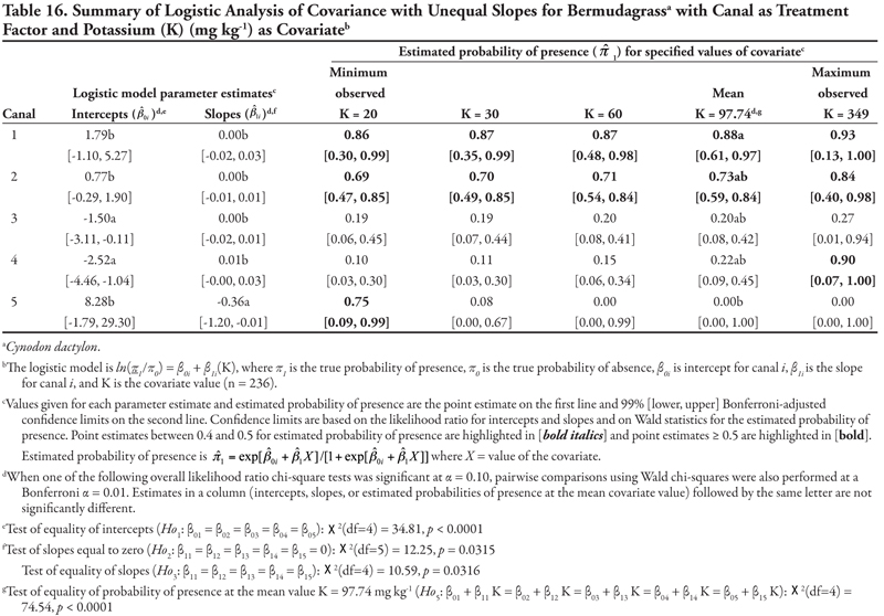
Canal as treatment factor: The two significant soil characteristic covariates for bermudagrass were K with unequal slope ANCOVA (Table 16, Figure 1D) and P with equal slope ANCOVA (Table 17). For K as a covariate, intercepts were significantly different from each other (p < 0.0001). The statistically negative intercepts for canal categories 3 and 4 indicated a low probability of occurrence if K = 0 for these smaller canals. Slopes were statistically not equal (p = 0.0316). As evidenced by the conservative 99% confidence intervals, only the slope for canal category 5 was significantly negative, while all remaining slopes were not different from zero. The predicted probability of bermudagrass presence was 0.75 at the minimum observed K (20 mg kg-1), but decreased rapidly as K increased for the smallest canal category. In contrast, the predicted probability for the first four canal categories did not change statistically as K increased. On the whole, bermudagrass was most likely to occur on the Leasburg Canal (category 1, ![]() ≥ 0.86) and on canals in category 2 (
≥ 0.86) and on canals in category 2 (![]() ≥ 0.69) regardless of the K concentration, and on canals in the smallest category (canal 5) at the minimum observed K = 20 mg kg-1 (
≥ 0.69) regardless of the K concentration, and on canals in the smallest category (canal 5) at the minimum observed K = 20 mg kg-1 (![]() = 0.75).
= 0.75).
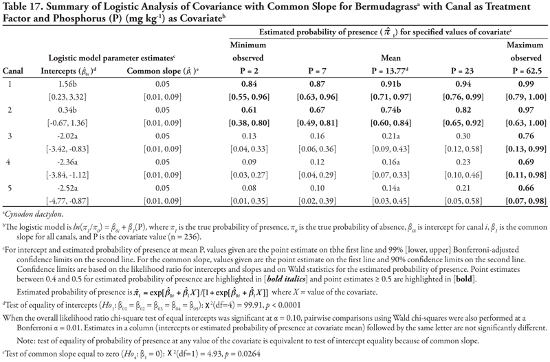
For P as a covariate (Table 17, Figure 1B), intercepts were statistically different (p < 0.0001) and decreased as canal size decreased. Specifically, the intercept for canal category 1 was statistically positive while the intercept for canal category 2 was not different from zero, and intercepts for canal categories 3, 4, and 5 were statistically negative, as evidenced by the 99% confidence interval. This result indicated that if P = 0, the highest probability of bermudagrass presence occurred for canal 1 (estimated logit = 1.56, ![]() = 0.83) and the lowest occurred for the three smallest canal categories (estimated logit < −2.02,
= 0.83) and the lowest occurred for the three smallest canal categories (estimated logit < −2.02, ![]() < 0.12). Similar to what was observed for K concentration, bermudagrass was predicted to occur more frequently on canals in categories 1 and 2 over all levels of P. However, bermudagrass was also predicted to occur more frequently (
< 0.12). Similar to what was observed for K concentration, bermudagrass was predicted to occur more frequently on canals in categories 1 and 2 over all levels of P. However, bermudagrass was also predicted to occur more frequently (![]() > 0.66) at the maximum observed P = 62.5 mg kg-1 on the smaller canals, although the prediction of bermudagrass presence at high values of P is not reliable due to the limited number of observations and wide confidence intervals.
> 0.66) at the maximum observed P = 62.5 mg kg-1 on the smaller canals, although the prediction of bermudagrass presence at high values of P is not reliable due to the limited number of observations and wide confidence intervals.
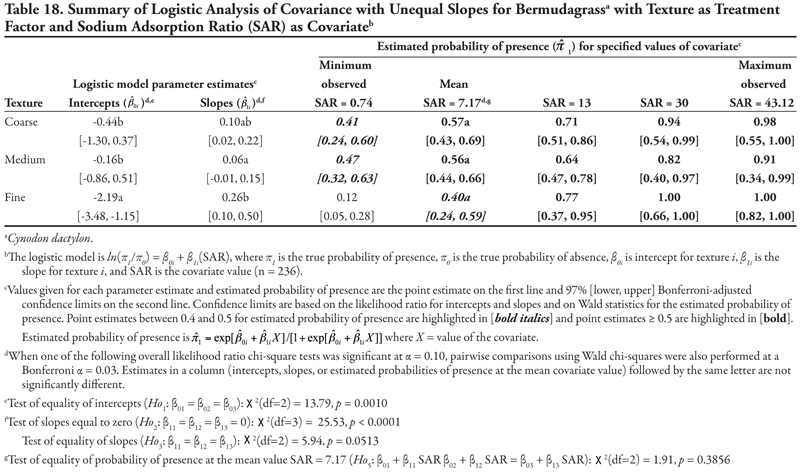
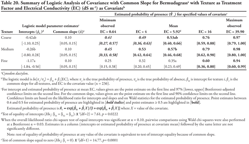
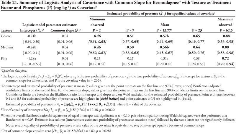
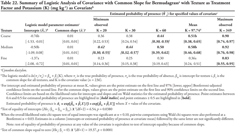
Soil texture as treatment factor: Bermudagrass had two significant soil characteristic covariates with unequal slope (SAR and OM, Tables 18 and 19, respectively) and three covariates with equal slope (EC, P, and K, Tables 20, 21, and 22, respectively). When SAR was the covariate (Table 18, Figure 1D), the intercept for fine texture was different from those of coarse and medium textures (p = 0.001). The negative intercept for fine texture indicated a low probability of bermudagrass presence if SAR = 0 (estimated logit = −2.19, ![]() = 0.10). Slopes were statistically different (p = 0.0513) and significantly positive, except for medium texture, for which the 97% confidence interval contained zero. As a result, a plot for Table 18 would resemble Figure 1D. With respect to the predicted probability of presence, bermudagrass was expected to occur at a probability greater than 0.4 regardless of soil texture or SAR level, except for fine-textured soils at the minimum SAR = 0.74. As SAR increased above 13, probability of bermudagrass presence increased regardless of soil texture. At the mean observed value SAR = 7.17, probability of occurrence was not significantly different among textures (p = 0.3856).
= 0.10). Slopes were statistically different (p = 0.0513) and significantly positive, except for medium texture, for which the 97% confidence interval contained zero. As a result, a plot for Table 18 would resemble Figure 1D. With respect to the predicted probability of presence, bermudagrass was expected to occur at a probability greater than 0.4 regardless of soil texture or SAR level, except for fine-textured soils at the minimum SAR = 0.74. As SAR increased above 13, probability of bermudagrass presence increased regardless of soil texture. At the mean observed value SAR = 7.17, probability of occurrence was not significantly different among textures (p = 0.3856).
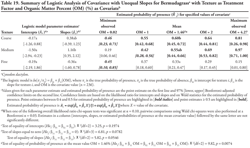
For the ANCOVA with OM as a covariate (Table 19, Figure 1C), intercepts were not different from each other (p = 0.1974), although medium texture had a statistically negative intercept, indicating low probability of presence if OM = 0. Slopes were statistically different (p = 0.0546), with medium texture having a positive slope while slopes for coarse- and fine-textured soils were not different from zero, as indicated by the 97% confidence intervals. This results in a plot like Figure 1C. With regards to probability of presence, as OM increased, predicted probabilities of bermudagrass presence increased in coarse- and medium-textured soils, but decreased in fine-textured soils. The probability of bermudagrass presence was greater than 0.4 for all levels of organic matter in coarse-textured soils, for OM > 1% in medium-textured soils, and only at the minimum OM = 0.02% in fine-textured soils.
When either EC or P was the covariate, intercepts were statistically different from each other (p = 0.0222 and p = 0.0020, Tables 20 and 21, respectively, Figure 1B), with fine texture having a significant negative intercept. A similar pattern for these two covariates was also seen in the significantly positive common slopes and consequent increase in probability of bermudagrass presence as either EC or P increased. At the mean observed value EC = 5.92 dS m-1 and P = 13.77 mg kg-1, coarse and medium textures had the highest estimated probability of presence (![]() ≥ 0.53 and
≥ 0.53 and ![]() ≥ 0.56, respectively). Probability of observing bermudagrass was again greater than 0.4 for all levels of EC and P in coarse- and medium-textured soils, while only at the highest level of EC or P in fine-textured soils. When K was the covariate (Table 22, Figure 1B), a similar pattern was observed, except that the intercept for coarse texture was also significantly negative. Again, similar to mean EC and P, at the observed mean K = 97.74 mg kg-1, bermudagrass was predicted to occur most frequently on medium- and coarse-textured soils.
≥ 0.56, respectively). Probability of observing bermudagrass was again greater than 0.4 for all levels of EC and P in coarse- and medium-textured soils, while only at the highest level of EC or P in fine-textured soils. When K was the covariate (Table 22, Figure 1B), a similar pattern was observed, except that the intercept for coarse texture was also significantly negative. Again, similar to mean EC and P, at the observed mean K = 97.74 mg kg-1, bermudagrass was predicted to occur most frequently on medium- and coarse-textured soils.
Rice cutgrass
Rice cutgrass is a cool-season creeping perennial that reproduces by rhizomes and seed (Darris and Bartow, 2006). This native species is most commonly found in moist wetland environments. It is a valuable food source for birds and small mammals and has been used in wetlands restoration and erosion control in ditches; however, the plant may not persist well after establishment. This species was found most frequently on the Leasburg canal in soils with higher OM content, and never occurred in samples taken on the smallest canals (category 5). The plant appeared to tolerate high sodicity and K, while pH, EC, or P concentration had no effect on presence; however, these results would require further study for confirmation. The potential for this species to be used in canal bank stabilization and restoration would also need further study.
Canal category as treatment factor: Over the 236 sampled locations of the study, rice cutgrass was only observed on canal categories 1, 2, 3, and 4 and had only one significant soil characteristic covariate, OM, with unequal slopes (Table 23, Figure 1C). Intercepts were not statistically different from one another (p = 0.5881), and only the intercepts for canal categories 1 and 2 were significantly negative, indicating a low probability of rice cutgrass presence if OM = 0. Slopes were different (p = 0.0239), with canal category 1 (Leasburg) having a statistically positive slope while slopes for the other three canal categories were not different from zero, as evidenced by the Bonferroni-adjusted 98.3% confidence intervals. With regards to the predicted probability of presence, as OM increased, rice cutgrass was expected to occur more frequently on the Leasburg Canal (category 1), but less frequently on canals in categories 2 and 3, and with very low probability on canals in category 4. However, the wide 98.3% confidence intervals at the maximum OM indicate unreliable probability estimates for canals in categories 2, 3 and 4 due to small sample sizes. Overall, rice cutgrass would be found more often (probability > 0.5) on the Leasburg Canal (category 1) in sections where OM content of the soils was greater than 1.45% than on any other canal of the system.
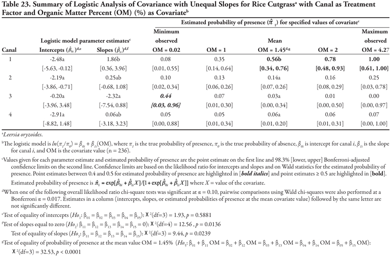
Texture as treatment factor: Rice cutgrass had two significant soil characteristic covariates with unequal slopes (SAR and K, Tables 24 and 25, respectively, Figure 1D) and two covariates with equal slope (OM and NO3-N, Tables 26 and 27, respectively, Figure 1A). For SAR ANCOVA, intercepts were different from each other (p = 0.0236), but were all significantly negative, indicating low probability of presence (![]() < 0.18) if SAR = 0 (Table 24). Slopes were significantly different (p = 0.0177). Only the slope for fine-textured soil was significantly positive, while slopes for the other two texture categories were not statistically different from zero, as indicated by the 97% confidence intervals. With regard to predicted probability of presence, rice cutgrass tended to occur more frequently as SAR increased. However, the large confidence intervals at high SAR for coarse and medium soil texture again indicate unreliability of the probability estimates. At the mean observed SAR = 7.17, textures were not different (p = 0.5403) for rice cutgrass presence. Rice cutgrass was only predicted to be found at probabilities greater than 0.5 on fine-textured soils with SAR > 30. A very similar pattern was observed for K (Table 25). Probability of observing rice cutgrass was low (
< 0.18) if SAR = 0 (Table 24). Slopes were significantly different (p = 0.0177). Only the slope for fine-textured soil was significantly positive, while slopes for the other two texture categories were not statistically different from zero, as indicated by the 97% confidence intervals. With regard to predicted probability of presence, rice cutgrass tended to occur more frequently as SAR increased. However, the large confidence intervals at high SAR for coarse and medium soil texture again indicate unreliability of the probability estimates. At the mean observed SAR = 7.17, textures were not different (p = 0.5403) for rice cutgrass presence. Rice cutgrass was only predicted to be found at probabilities greater than 0.5 on fine-textured soils with SAR > 30. A very similar pattern was observed for K (Table 25). Probability of observing rice cutgrass was low (![]() < 0.20) except when K levels were very high (> 97.74 mg kg-1), especially in medium- and fine-textured soils.
< 0.20) except when K levels were very high (> 97.74 mg kg-1), especially in medium- and fine-textured soils.
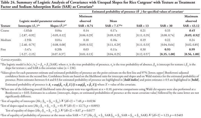
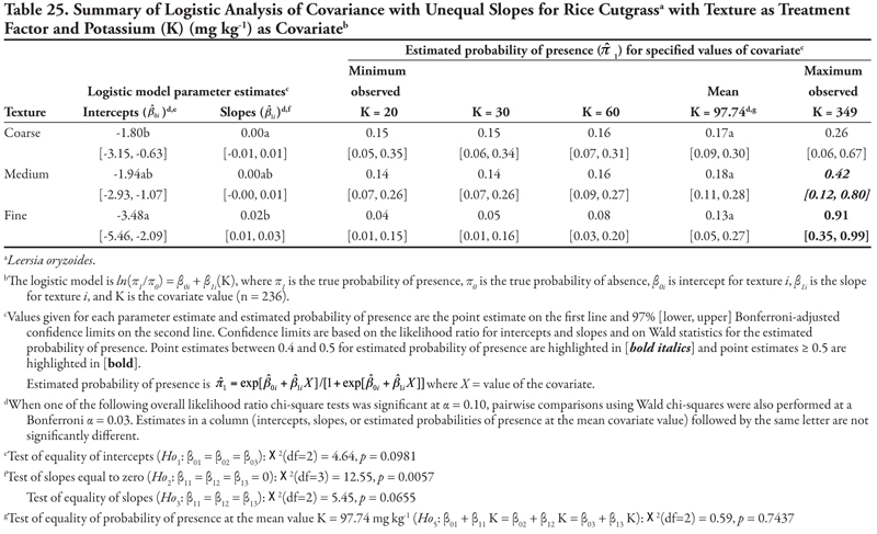
For OM as a covariate, intercepts were not significantly different (p = 0.2966) and were all significantly negative (Table 26), indicating a very low probability of presence if OM = 0, similar to SAR and K. The common slope was significantly positive (p = 0.0377), resulting in a plot like Figure 1A. For the predicted probability of presence, rice cutgrass occurred most frequently on soils of all textures with high OM and least frequently where OM was low. When NO3-N was evaluated as a covariate (Table 27), the pattern was similar to that of OM except that the common slope was significantly negative. As a result, probability of rice cutgrass presence decreased as NO3-N increased regardless of soil texture.
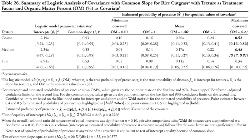
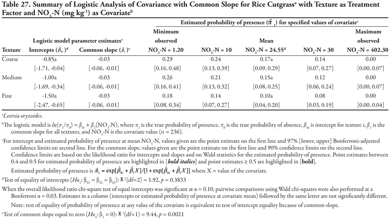
Johnsongrass
Johnsongrass is an invasive, creeping perennial weed that reproduces vegetatively by rhizomes and by seed (DiTomaso and Healy, 2007). It is a major weed of disturbed sites and cultivated crops and is a state-listed noxious weed in many western states. Johnsongrass habitat also includes orchards and ditchbanks, and it grows well on moist soils. The results described below also suggest that Johnsongrass may tolerate saline soils; this characteristic would make this species more competitive in many NM soils and should be a topic for further study. Johnsongrass presence was not affected by soil SAR, OM, NO3-N, P, or K in this survey.
Canal category as treatment factor: Johnsongrass had two significant soil characteristic covariates (pH and EC), the effects of which were consistent over canal category, resulting in logistic ANCOVA models with common slope (Tables 28 and 29, respectively, Figure 1B). For the pH ANCOVA, intercepts were statistically different (p = 0.0594), but only intercepts for canal categories 2 and 3 were significant and positive (Table 28), indicating the high probability of presence if pH = 0 with the highest probability of ![]() = 1.00 for canals in category 3 (estimated logit = 24.44). The common slope was significantly negative (p = 0.0057), resulting in the decrease in predicted probability of Johnsongrass presence over all canal categories as pH increased. With the consistent effect over canal categories, Johnsongrass was most likely to occur on canals in category 3 followed by canals in category 2, and was least likely to occur on canals in category 4. The probability of presence was greater than 0.4 only for canal categories 2 and 3 at the minimum observed pH = 7.25.
= 1.00 for canals in category 3 (estimated logit = 24.44). The common slope was significantly negative (p = 0.0057), resulting in the decrease in predicted probability of Johnsongrass presence over all canal categories as pH increased. With the consistent effect over canal categories, Johnsongrass was most likely to occur on canals in category 3 followed by canals in category 2, and was least likely to occur on canals in category 4. The probability of presence was greater than 0.4 only for canal categories 2 and 3 at the minimum observed pH = 7.25.
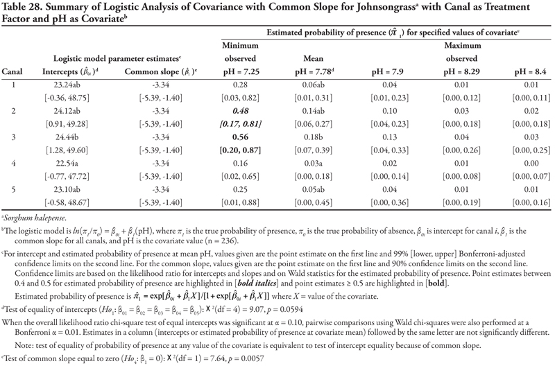
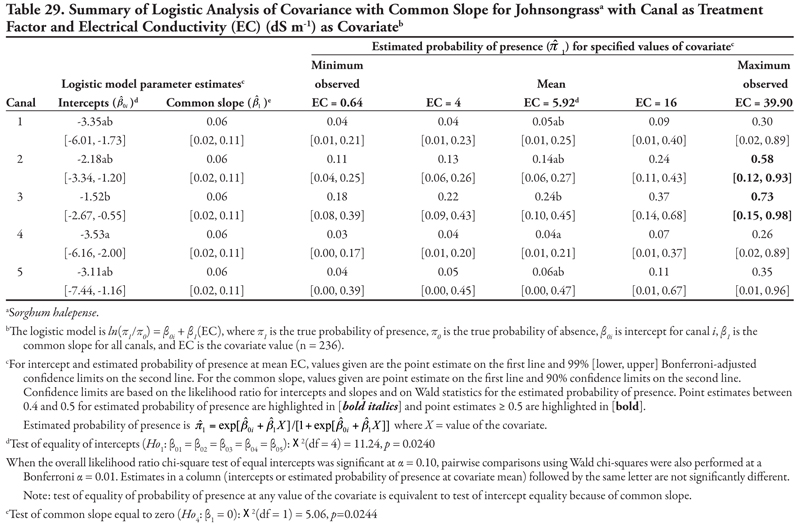
When EC was the covariate, intercepts were significantly different (p = 0.0240) and were all statistically negative (Table 29), indicating a low probability of presence if EC = 0 (![]() < 0.18). With the common positive slope (p = 0.0244), the probability of presence increased as EC increased. It reached its highest probability for each canal category at the maximum observed EC of 39.90 dS m-1. However, these estimates were unreliable because of small sample sizes. At the mean EC = 5.92 dS m-1, the probability of Johnsongrass presence was highest on canal category 3 and lowest on canal category 4. Johnsongrass was not found regularly on any canal, but analyses predicted that this species would be found most often on canals in category 3 on soils with high EC.
< 0.18). With the common positive slope (p = 0.0244), the probability of presence increased as EC increased. It reached its highest probability for each canal category at the maximum observed EC of 39.90 dS m-1. However, these estimates were unreliable because of small sample sizes. At the mean EC = 5.92 dS m-1, the probability of Johnsongrass presence was highest on canal category 3 and lowest on canal category 4. Johnsongrass was not found regularly on any canal, but analyses predicted that this species would be found most often on canals in category 3 on soils with high EC.
Texture as treatment factor: When texture was the treatment factor, Johnsongrass had only pH as a significant covariate with a common negative slope (Table 30, Figure 1B). Intercepts were significantly different but all positive, indicating a high probability of presence if pH = 0. As a result of negative slope, predicted probability of Johnsongrass presence decreased as pH increased. Overall, Johnsongrass occurred most frequently on coarse-textured soil with pH = 7.25 (minimum observed pH) and least frequently on fine-textured soil.
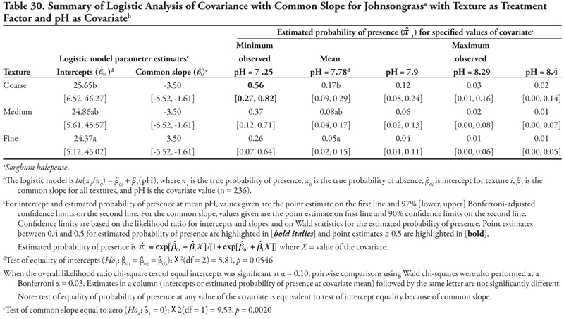
Echinochloa species
These nonnative, summer annual grasses are found nearly worldwide and are common weed problems in agricultural lands (DiTomaso and Healy, 2007). The seed of barnyardgrass (Echinochloa crus-galli) can float on water for several days, indicating that presence on the canals may increase the infestation of these species in nearby agricultural production fields. The recorded habitat for these species also includes ditches and margins of ponds and suggests that the presence of these species on the canals would be expected; however, further work is needed to understand why these plants were most common on canals of category 4 and on fine-textured soils at increasing P concentrations in this survey. The soil characteristics pH, EC, NO3-N, and K had no effect on Echinochloa spp. presence in this survey.
Canal category as treatment factor: In testing the null hypothesis of covariate slope equal to zero (Ho2), none of the soil covariates was significant for Echinochloa spp. (E. crus-galli and E. colona) when canal was the treatment factor (data not shown). Therefore, ANOVA results are summarized in Table 31 (Figure 2B) for the logistic ANOVA model for Echinochloa spp. The canal p-value for testing equality of canal means (Ho6) was < 0.0001, so at α = 0.10, we reject the null hypothesis that the five canal categories have equal probability of presence of Echinochloa spp. The estimated probability of Echinochloa spp. presence was lowest for the largest canal category 1 (0.03), higher for canals in categories 2 and 3 (0.31, 0.35), highest for canals in category 4 (0.51), then decreased for the smallest canal category 5 (0.14). Therefore, Echinochloa spp. would most likely be observed on canals from category 4.
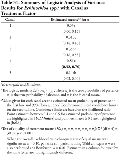
Texture as treatment factor: Echinochloa spp. had one significant soil characteristic covariate with unequal slopes (P, Table 32, Figure 1C) and two covariates with common slope (SAR and OM, Tables 33 and 34, respectively). For P ANCOVA, intercepts were not different from each other (p = 0.2697). Only the intercept for fine soil texture was significant and negative, indicating a low probability of presence if P = 0. Slopes were significantly different from each other (p = 0.07). Note that the conservative 97% Bonferroni-adjusted confidence intervals incorrectly indicate that all slopes are not statistically different from zero. However, the slope for fine-textured soil was positive, while slopes for coarse and medium soil textures were not different from zero. Medium-textured soil slope was not different from that of fine-textured. Therefore, as P increased, predicted probability of Echinochloa spp. presence tended to decrease in soils with coarse and medium texture but to increase in fine-textured soil. At mean P = 13.77 mg kg-1, the probability of presence of Echinochloa spp. was not significantly different across soil textures (p = 0.5280). The only situation where the probability of finding Echinochloa spp. was greater than 0.5 was on fine-textured soil where P = 62.5 mg kg-1.
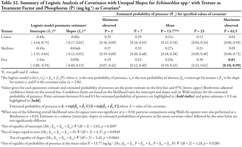
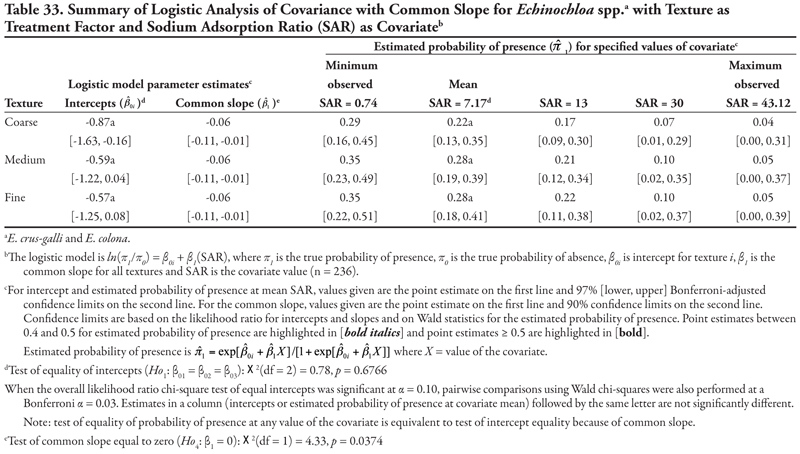
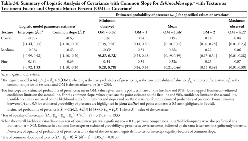
When SAR was evaluated as a covariate in logit ANCOVA, intercepts were not significantly different, while the common slope was statistically negative (p = 0.0374, Table 33, Figure 1A). Therefore, Echinochloa spp. were predicted to occur less frequently as SAR increased. The probability of finding these species was low (< 0.4) on all soil textures and SAR levels. A similar pattern was observed for OM (Table 34). Echinochloa spp. were predicted to be present at probabilities greater than 0.4 only on medium- and fine-textured soils with OM = 0.02%.
Plantago species
The plantains are perennial broadleaf (sometimes annual or biennial) plants that reproduce only by seed (DiTomaso and Healy, 2007). They are commonly found in disturbed places, although irrigation ditches or ditchbanks are not listed as common habitat. The seed will disperse with water, indicating that they may persist once established on the canals. In addition, occasional mowing (a common management practice on the canals) may favor survival of these plants. The results of the survey suggest that while soil texture does not influence presence, plantains may be able to survive in saline or sodic soils. The remaining soil characteristics, pH, OM, NO3-N, P, or K, had no effect on plantain presence in this survey.
Canal category as treatment factor: Plantago spp. (P. lanceolata and P. major) had two significant soil characteristic covariates (EC and SAR), the effects of which were not consistent over canals, resulting in logistic ANCOVA models with unequal slopes (Tables 35 and 36, respectively, Figure 1D). In both models, only intercepts for canal categories 3 and 4 were significantly negative. Covariate slopes were different from zero (p = 0.0190 for EC and p = 0.0465 for SAR). Note that the conservative 97% Bonferroni-adjusted confidence intervals incorrectly indicate all slopes are not statistically different from zero for both EC and SAR models. At mean EC = 5.92 dS m-1 and SAR = 7.17, Plantago spp. were most likely to occur on canals in category 5 and least likely to occur on canal category 1 (i.e., Leasburg canal). Except for the largest canal, where the probability of presence decreased, Plantago spp. were more likely to occur as EC or SAR increased. However, the estimated probabilities for these species were unreliable over all values of EC and SAR, as indicated by the wide 99% confidence intervals, because Plantago spp. were relatively rare on canals in categories 1 and 5 and at high levels of EC or SAR. Among the other canal categories, Plantago spp. were more likely to occur on canals in category 2 at all values of EC or SAR ( ![]() > 0.40) and on canals in categories 3 and 4 at EC > 16 dS m-1 or SAR > 13.
> 0.40) and on canals in categories 3 and 4 at EC > 16 dS m-1 or SAR > 13.
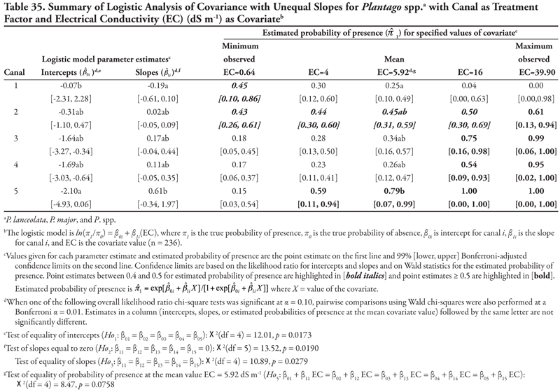
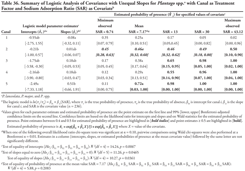
Texture as treatment factor: Similar to Echinochloa spp. with canal as the treatment factor, none of the soil covariates for Plantago spp. was significant in the test of slopes equal to zero (Ho2) when texture was the treatment factor. The logistic ANOVA model for Plantago spp. with texture as treatment factor was, therefore, summarized in an ANOVA table (Table 37, Figure 2A). The test of equality of treatment means (Ho6) resulted in a p-value = 0.4878. Hence, at α = 0.10, we fail to reject the above null hypothesis and conclude that probability of Plantago spp. presence was the same for all soil textures, with Plantago spp. occurring at about 34% of locations on average (Table 3).
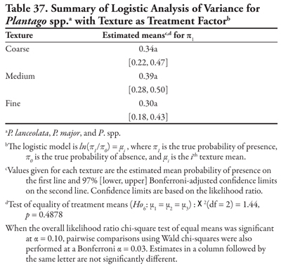
Curly dock
Curly dock (Rumex crispus) is a nonnative perennial broadleaf weed that reproduces by seed (DiTomaso and Healy, 2007). The habitat for this species includes disturbed moist sites, such as ditches and wetlands, as well as in perennial agronomic crops such as alfalfa. The fruit are winged, which provides buoyancy in flowing water for effective dispersal of seed. The survey results were very unclear, possibly due to the limited number of observations. However, the results suggest that further work should concentrate sample collection on smaller canals and should determine the effect of saline soil and NO3-N on presence of this species. The results also suggest that curly dock presence on the canals is not affected by P or K concentration in soil.
Canal category as treatment factor: Curly dock had three significant soil characteristic covariates, EC, SAR, and OM, with unequal slopes (Tables 38, 39, and 40, respectively). When EC was the covariate (Table 38), intercepts were different (p = 0.0009), but only the intercept for canal category 2 was significant and negative, indicating a low probability of presence if EC = 0 (estimated logit = −2.26, ![]() = 0.09). The slope for canal category 5 was significantly negative, while slopes for the other four canal categories were not different from zero, as evidenced by the 99% confidence intervals. At mean EC = 5.92 dS m-1, estimated probability of presence was not statistically different over canal categories (p = 0.2314). Generally, probability estimates of curly dock presence over different values of EC in canal category 5 and at the maximum observed EC for all canal categories were unreliable (as indicated by the wide 99% intervals as a result of small sample size) and erratic, as evidenced by the fact that the highest probability for observing curly dock occurred on canal category 2 at the maximum observed EC (72%) and at the lowest observed EC (86%) on canal category 5.
= 0.09). The slope for canal category 5 was significantly negative, while slopes for the other four canal categories were not different from zero, as evidenced by the 99% confidence intervals. At mean EC = 5.92 dS m-1, estimated probability of presence was not statistically different over canal categories (p = 0.2314). Generally, probability estimates of curly dock presence over different values of EC in canal category 5 and at the maximum observed EC for all canal categories were unreliable (as indicated by the wide 99% intervals as a result of small sample size) and erratic, as evidenced by the fact that the highest probability for observing curly dock occurred on canal category 2 at the maximum observed EC (72%) and at the lowest observed EC (86%) on canal category 5.
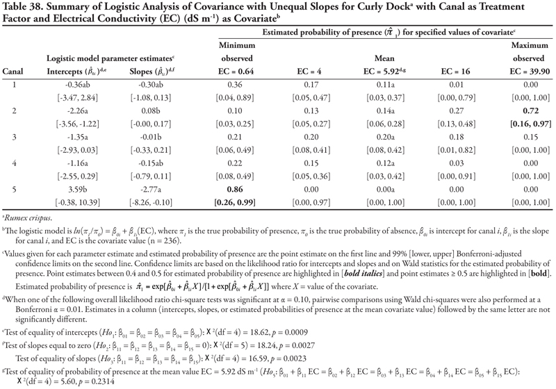
The ANCOVA results for SAR as covariate were inconsistent, making the choice of a model somewhat subjective. First, the unequal slopes case (Table 39) showed that the null hypothesis of slopes equal to zero (Ho2) was rejected (p = 0.0763) and that the test of equal slopes (Ho3) was not rejected (p = 0.1101). Therefore, a common slope ANCOVA was fitted. For this analysis (data not shown), the test of common slope equal to zero (Ho4) was not rejected (p = 0.1086), implying that an ANOVA model with no covariate was appropriate, which contradicted the results of the unequal slopes ANCOVA. We decided to report the results of the unequal slopes ANCOVA (Table 39), but these results must be treated with caution and may be due to curly dock being relatively rare on canals in categories 1 and 5 and at high SAR (similar to the pattern with Plantago spp.). For example, 99% confidence intervals for estimated probability of presence are very wide except for (possibly) canal categories 1 to 4 at mean SAR = 7.17. Even these confidence intervals are fairly wide. In addition, the conservative 97% Bonferroni-adjusted confidence intervals on the slopes incorrectly indicate that all slopes are not statistically different from zero.
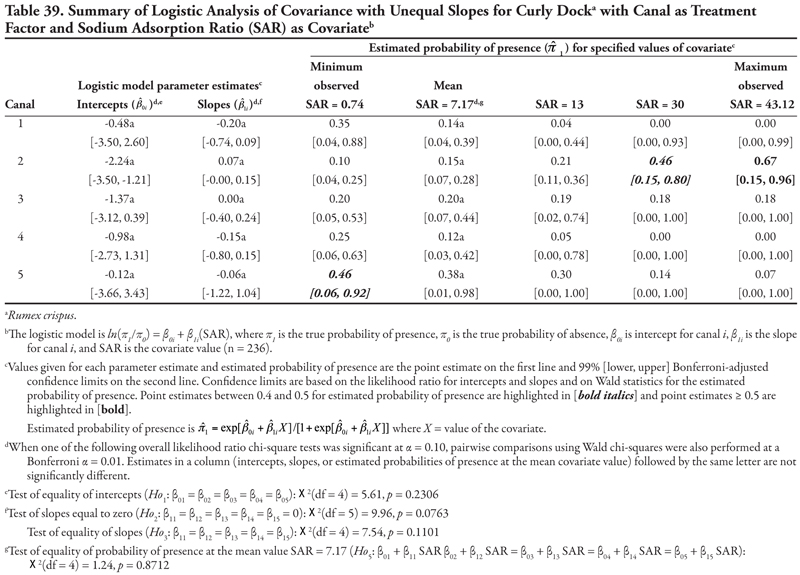
For OM ANCOVA, intercepts were different (p = 0.0424) and intercepts for canal categories 3 and 4 were significantly negative, indicating low probability of presence if OM = 0 (Table 40). If OM = 0, the lowest probability of curly dock presence was for canal category 4 with estimated logit of −5.12 and ![]() = 0.01. As OM increased, curly dock occurred more frequently on the three smallest canal categories and occurred less frequently on the two larger canal categories. However, at the maximum observed OM = 4.27%, the wide 99% confidence intervals for the estimated probabilities implied unreliable estimates due to small sample size.
= 0.01. As OM increased, curly dock occurred more frequently on the three smallest canal categories and occurred less frequently on the two larger canal categories. However, at the maximum observed OM = 4.27%, the wide 99% confidence intervals for the estimated probabilities implied unreliable estimates due to small sample size.
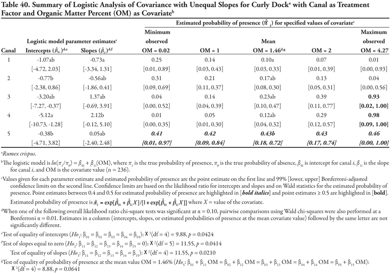
Texture as treatment factor: Curly dock had two significant soil characteristic covariates (pH and NO3-N), the effects of which were not consistent across soil textures, resulting in logistic ANCOVA models with unequal slopes (Tables 41 and 42, respectively, Figure 1D). For pH ANCOVA, only the intercept for the medium texture category was significant and negative, as evidenced by the confidence intervals (Table 41), but all three intercepts had very wide confidence intervals, indicating unreliable estimates if pH = 0. Only the slope for the medium texture category was significant and positive, and slope confidence intervals were also wide. The probability of presence for these textures increased as pH increased for medium and fine soil texture, but curly dock was less likely to occur as pH increased in the coarse-textured soil. At the mean observed pH = 7.78, estimated probabilities of curly dock presence in different textures were significantly different from each other (p = 0.0781), with curly dock most likely to occur on fine-textured soil.
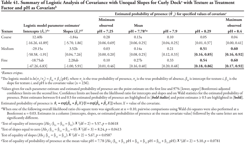
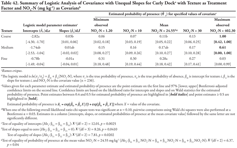
When NO3-N was evaluated as a covariate, all intercepts were significantly negative, indicating low probability of presence if NO3-N = 0 (Table 42). Only the slope for coarse-textured soil was significant and positive, while slopes for the other two textures were not different from zero. With regards to predicted probability of presence, as NO3-N increased, curly dock occurred more frequently in soils with coarse and medium texture but less frequently in fine soil texture.
Acknowledgements
The Rio Grande Basin Initiative provided the funding to accomplish the research reported here. The authors are grateful for the cooperation of the Elephant Butte Irrigation District by granting permission to access the irrigation canals. Undergraduate and graduate student workers provided much needed assistance to the project; the authors would like to thank Sara Schuster in particular for her assistance during sampling.
References
Aldrich, R.J., and R.J. Kremer. 1997. Principles in weed management, 2nd ed. Ames: Iowa State University Press.
Darris, D., and A. Bartow. 2006. Rice cutgrass [Online]. Corvalis, OR: U.S. Department of Agriculture, Natural Resources Conservation Service, Plant Materials Center. Retrieved July 15, 2010, from http://plants.usda.gov/factsheet/pdf/fs_leor.pdf.
DiTomaso, J.M., and E.A. Healy. 2007. Weeds of California and other western states, vol. 1 and 2 [Agriculture and Natural Resources Publication 3488]. Davis: University of California.
Dowdy, S., and S. Wearden. 1991. Statistics for research. New York: John Wiley & Sons.
Elephant Butte Irrigation District. 1998. General data and information [Online]. Retrieved October 31, 2006, from http://www.ebid-nm.org//static/PDF/EBIDBOOK-2.pdf.
Fiore, C., X. Liu, J. Schroeder, S. Schuster, L. Murray, R. Sanderson, M. Renz, A. Ulery, and O. El-Sebai. 2006. Vegetation on irrigation canals in southern New Mexico. Proceedings of the Western Society of Weed Science, 59, 46.
Gavlak, R., D. Horneck, R.O. Miller, and J. Kotuby-Amacher. 2003. Soil, plant and water reference methods for the Western Region, 2nd ed. Western Regional Extension Publication 125.
Herrera, E. 2000. Soil test interpretations [Guide A-122]. Las Cruces: New Mexico State University Cooperative Extension Service.
Kutner, M.H., C.J. Nachtsheim, and J. Neter. 2004. Applied linear regression models, 4th ed. New York: McGraw-Hill/Irwin.
McCullagh, P., and J. Nelder. 1983. Generalized linear models. London: Chapman Hall.
Ross, M.A., and C.A. Lembi. 2009. Applied weed science including the ecology and management of invasive plants, 3rd ed. Upper Saddle River, NJ: Pearson Prentice Hall.
SAS Institute Inc. 2004. SAS/STAT® 9.1 User’s Guide. Cary, NC: SAS Institute Inc.
Schuster, S., D. Cowley, C. Fiore, L. Murray, and J. Schroeder. 2004. Are weed species associated with crayfish habitat along the irrigation canals? Proceedings of the Western Society of Weed Science, 57, 37.
U.S. Department of the Interior, Bureau of Reclamation. 2003. Rio Grande Project [Online]. Retrieved September 20, 2006, from http://www.usbr.gov/projects/Project.jsp?proj_Name=Rio+Grande+Project.
Appendices
Appendix A-1. Map of the 299 randomly selected sampling locations along the Leasburg/Las Cruces/Mesilla canal system.
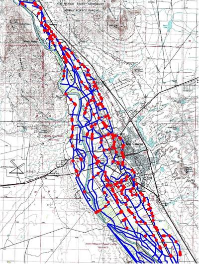
Appendix A-2. Canals of the Leasburg System as Categorized for the Vegetation Survey (EBID, 1998)
| Canal Category | Canal Name | Canal Category | Canal Name |
| 1 | Leasburg Canal | 4 | Picacho A Lateral |
| 2 | Las Cruces Canal | 4 | Picacho C Lateral |
| 2 | Armijo Lateral | 4 | School Lateral |
| 2 | Mesilla Canal | 4 | Nusbaum Lateral |
| 2 | Picacho Main Lateral | 5 | Arguelles Lateral |
| 3 | Doña Ana Lateral | 5 | Seldon Lateral |
| 3 | Clark Lateral | 5 | Hare Lateral |
| 3 | Laguna Lateral | 5 | Arrington Lateral |
| 3 | Louisiana Lateral | 5 | Rio Rancho Lateral |
| 3 | California Lateral | 5 | Propeck Lateral |
| 3 | Middle Lateral | 5 | Etajo Lateral |
| 4 | Baca Lateral | 5 | Barrio Lateral |
| 4 | Kerr Lateral | 5 | Kelso Lateral |
| 4 | American Bend Lateral | 5 | Cooney Lateral |
| 4 | Hill Lateral | 5 | Anderson Lateral |
| 4 | Taylor Lateral | 5 | Redd Lateral |
| 4 | Elwood Lateral | 5 | Mayfield Lateral |
| 4 | Crapps Lateral | 5 | Porter Lateral |
| 4 | Quesenberry Lateral | 5 | Turney Lateral |
| 4 | Tortugas Lateral | 5 | Utting Lateral |
| 4 | Houghton Lateral | 5 | Alamo Lateral |
| 4 | Apache Lateral | 5 | Gardner Lateral |
| 4 | Longwell Lateral | 5 | College Lateral |
| 4 | Gillen Lateral | 5 | Corralitos Lateral |
| 4 | California Ext. Lateral | 5 | Lester Lateral |
| 4 | Williams Lateral | 5 | Goering Lateral |
| 4 | Freudenthal Lateral |
Appendix A-3. Distribution of three categories of soil texture along the five categories of canal capacity in the Leasburg canal system of the EBID.
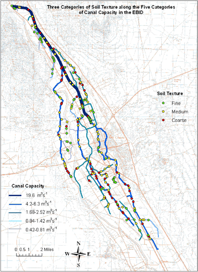
Appendix B. Rio Grande Basin Initiative, Environmental Data, Leasburg Weather Station (elevation 1,215 m; latitude 32° 29’ 46.68” N, longitude 106° 55’ 49.44” W; as reported at http://weather.nmsu.edu)
| Year | Month | Air Temperature (°C) | Precipitation Monthly Total (cm) |
||
| MIN | MEAN | MAX | |||
| 2002 | January | −2.8 | 6.1 | 16.0 | 0.58 |
| 2002 | February | −1.7 | 7.5 | 16.7 | 1.78 |
| 2002 | March | 1.4 | 12.4 | 22.2 | 0.00 |
| 2002 | April | 9.1 | 20.2 | 29.6 | 0.00 |
| 2002 | May | 10.7 | 22.7 | 32.5 | 0.05 |
| 2002 | June | 17.8 | 28.8 | 38.1 | 0.05 |
| 2002 | July | 19.5 | 26.7 | 34.9 | 1.63 |
| 2002 | August | 18.3 | 26.9 | 36.3 | 5.66 |
| 2002 | September | 15.1 | 23.5 | 32.4 | 1.37 |
| 2002 | October | 8.0 | 16.1 | 25.0 | 1.83 |
| 2002 | November | 0.8 | 9.4 | 19.0 | 0.94 |
| 2002 | December | −2.1 | 5.0 | 13.8 | 3.73 |
| 2003 | January | −2.0 | 7.7 | 19.3 | 0.00 |
| 2003 | February | 0.9 | 9.0 | 17.0 | 3.96 |
| 2003 | March | 2.2 | 11.8 | 21.1 | 0.36 |
| 2003 | April | 5.2 | 16.8 | 26.4 | 0.05 |
| 2003 | May | 11.7 | 23.0 | 32.5 | 0.00 |
| 2003 | June | 16.0 | 26.5 | 35.6 | 3.28 |
| 2003 | July | 20.3 | 29.2 | 37.8 | 0.58 |
| 2003 | August | 19.4 | 27.6 | 36.2 | 3.23 |
| 2003 | September | 15.4 | 24.3 | 33.2 | 0.33 |
| 2003 | October | 9.5 | 18.7 | 29.0 | 1.37 |
| 2003 | November | 1.4 | 10.6 | 20.2 | 1.55 |
| 2003 | December | −4.7 | 4.8 | 15.6 | 0.00 |
| 2004 | January | −1.6 | 6.7 | 15.6 | 0.86 |
| 2004 | February | −3.0 | 6.4 | 15.6 | 0.00 |
| 2004 | March | 5.1 | 14.2 | 23.4 | 1.91 |
| 2004 | April | 7.3 | 16.4 | 24.3 | 5.08 |
| 2004 | May | 12.0 | 23.2 | 32.5 | 0.00 |
| 2004 | June | 15.5 | 26.1 | 35.6 | 6.17 |
| 2004 | July | 18.6 | 27.3 | 36.1 | 1.09 |
| 2004 | August | 16.9 | 25.0 | 33.7 | 4.14 |
| 2004 | September | 13.5 | 21.8 | 30.7 | 4.98 |
| 2004 | October | 8.4 | 16.5 | 25.3 | 2.67 |
| 2004 | November | 1.2 | 8.3 | 16.5 | 3.99 |
| 2004 | December | −3.1 | 4.4 | 14.0 | 1.78 |
| 2005 | January | −0.4 | 7.4 | 16.5 | 2.72 |
| 2005 | February | 2.5 | 8.5 | 15.4 | 4.55 |
| 2005 | March | 2.8 | 11.5 | 19.9 | 0.89 |
| 2005 | April | 5.7 | 16.5 | 26.1 | 0.69 |
| 2005 | May | 11.2 | 22.3 | 31.7 | 1.68 |
| 2005 | June | 15.7 | 27.2 | 36.8 | 0.00 |
| 2005 | July | 19.2 | 28.9 | 38.0 | 1.91 |
| 2005 | August | 18.8 | 25.8 | 33.9 | 3.45 |
| 2005 | September | 15.5 | 24.2 | 33.4 | 3.99 |
| 2005 | October | 8.6 | 16.9 | 25.8 | 1.57 |
| 2005 | November | 0.2 | 10.7 | 22.4 | 0.00 |
| 2005 | December | −3.1 | 6.5 | 17.6 | 0.00 |
| 2006 | January | −3.5 | 7.0 | 18.2 | 0.13 |
| 2006 | February | −0.5 | 9.6 | 20.2 | 0.00 |
| 2006 | March | 3.7 | 13.1 | 22.1 | 0.13 |
| 2006 | April | 7.8 | 19.2 | 28.9 | 0.46 |
| 2006 | May | 12.7 | 24.4 | 33.9 | 0.81 |
| 2006 | June | 17.8 | 28.1 | 37.0 | 0.13 |
| 2006 | July | 20.3 | 27.9 | 36.0 | 2.08 |
| 2006 | August | 18.7 | 24.8 | 32.7 | 12.80 |
| 2006 | September | 15.5 | 20.5 | 26.9 | 11.51 |
EBID Irrigation Season
| Year | Dates | Dates | Sample Dates | |||
| Release | Shutdown | Release | Shutdown | First | Last | |
| 2002 | 2/19 | 10/11 | 7/25 | 9/26 | ||
| 2003 | 3/21 | 4/22 | 5/15 | 9/4 | 6/11 | 7/28 |
| 2004 | 3/15 | 4/12 | 5/22 | 9/19 | none | none |
| 2005 | 3/22 | 10/13 | 7/12 | 9/29 | ||
| 2006 | 3/15 | 10/12 | 6/30 | 8/17 | ||
Appendix C. Complete List of All 76 Observed Species and Groups of Species (in alphabetical order) with Number of Locations Where Present Out of 247 Total Sample Locations (species marked with * are on the NM noxious weed list)
| CODE | Scientific Name | Common Name | Number of Locations Where Present |
| ALYAL | Alyssum alyssoides | yellow alyssum | 1 |
| AMAPA | Amaranthus palmeri | Palmer amaranth | 19 |
| ANNBR | Annual broadleaf | unidentified species | 3 |
| ANVCR | Anoda cristata | spurred anoda | 8 |
| ASCSY | Asclepias syriaca | common milkweed | 1 |
| ASTSP | Asteraceae | sunflower family, unidentified species | 60 |
| ASTSN | Aster spinosus | spiny aster | 3 |
| BACGL | Baccharis glutinosa | seepwillow | 26 |
| BRASP | Brassicaceae | mustard family, unidentified species | 1 |
| BROCA | Bromus catharticus | rescuegrass | 2 |
| BROSP | Bromus spp. | unidentified species | 1 |
| BROTE | Bromus tectorum | downy brome | 3 |
| CCHIN | Cenchrus pauciflorus | field sandbur | 7 |
| CHEAL | Chenopodium album | common lambsquarters | 3 |
| CHRVI | Chloris virgata | feather fingergrass | 3 |
| CONAR | Convolvulus arvensis* | field bindweed | 9 |
| ERICA | Conyza canadensis | horseweed | 2 |
| CYNDA | Cynodon dactylon | bermudagrass | 126 |
| CYPES | Cyperus esculentus | yellow nutsedge | 48 |
| CYPRO | Cyperus rotundus | purple nutsedge | 12 |
| DIGSA | Digitaria sanguinalis | large crabgrass | 1 |
| DISSP | Distichlis spicata | saltgrass | 1 |
| ECHCG | Echinochloa crus-galli | barnyardgrass | 42 |
| ECHCO | Echinochloa colona | junglerice | 30 |
| ECHSP | Echinochloa spp. | unidentified species | 1 |
| EPHSP | Euphorbia spp.* | spurges | 10 |
| EQUHY | Equisetum hyemale | horsetail/scouringrush | 83 |
| ERBGR | Eriochloa gracilis | southwestern cupgrass | 8 |
| FABSP | Fabaceae | pea family, unidentified species | 3 |
| GAAPA | Gaura parviflora | smallflower gaura | 2 |
| HELCI | Helianthus ciliaris | Texas blueweed | 2 |
| HOFDE | Hoffmannseggia glauca | hogpotato | 8 |
| HORJU | Hordeum jubatum | foxtail barley | 21 |
| IPOHE | Ipomoea hederacea | ivyleaf morningglory | 1 |
| PHBPU | Ipomoea purpurea | tall morningglory | 2 |
| JUNSP | Juncus spp. | rush | 11 |
| KCHSC | Kochia scoparia | kochia | 13 |
| LEEOR | Leersia oryzoides | rice cutgrass | 39 |
| LEFFI | Leptochloa filiformis | red sprangletop | 1 |
| LEFSP | Leptochloa spp. | sprangletop | 1 |
| LEFUN | Leptochloa uninervia | Mexican sprangletop | 1 |
| LYGJU | Lygodesmia juncea | skeletonweed | 2 |
| MACCA | Machaeranthera canescens | purple aster | 2 |
| MALNE | Malva neglecta | common mallow | 3 |
| MEDSA | Medicago sativa | alfalfa | 2 |
| MIXED | Mixed | unidentified species | 119 |
| MUHAS | Muhlenbergia asperifolia | scratchgrass | 1 |
| OENBE | Oenothera berlandieri | Mexican evening primrose | 17 |
| PANDI | Panicum dichotomiflorum | fall panicum | 1 |
| PASDI | Paspalum dilatatum | dallisgrass | 10 |
| PHAMI | Phalaris minor | littleseed canarygrass | 1 |
| PHYNO | Phyla nodiflora | matchhead | 13 |
| PLALA | Plantago lanceolata | buckhorn plantain | 67 |
| PLAMA | Plantago major | broadleaf plantain | 14 |
| PLASP | Plantago spp. | plantain spp. | 4 |
| POASP | Poaceae | grass family, unidentified species | 19 |
| POLMO | Polypogon monspeliensis | rabbitfoot polypogon | 10 |
| POROL | Portulaca oleracea | common purslane | 11 |
| RUMCR | Rumex crispus | curly dock | 48 |
| SAZCY | Sarcostemma cynanchoides | climbing milkweed | 1 |
| SASKR | Salsola iberica | Russian thistle | 9 |
| SETLU | Setaria lutescens | yellow foxtail | 24 |
| SETVU | Setaria verticillata | bristly foxtail | 3 |
| SIDHE | Sida hederacea | alkali sida | 3 |
| SSYIR | Sisymbrium irio | London rocket | 1 |
| SOLEL | Solanum elaeagnifolium | silverleaf nightshade | 6 |
| SONOL | Sonchus oleraceus | annual sowthistle | 8 |
| SORHA | Sorghum halepense | Johnsongrass | 29 |
| SPHCO | Sphaeralcea coccinea | scarlet globemallow | 3 |
| TAROF | Taraxacum officinale | common dandelion | 2 |
| TRBTE | Tribulus terrestris | puncturevine | 7 |
| TRFRE | Trifolium repens L. | clover | 2 |
| TRTPO | Trianthema portulacastrum | horse purslane | 8 |
| TYHSP | Typha spp. | cattail | 1 |
| ULMPU | Ulmus pumila* | Siberian elm | 16 |
| VESTH | Verbascum thapsus | common mullein | 1 |
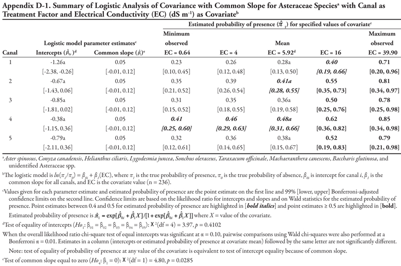
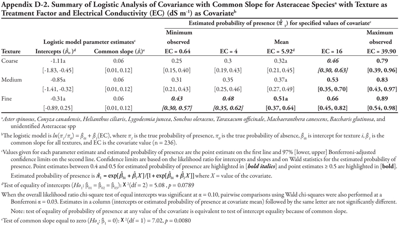
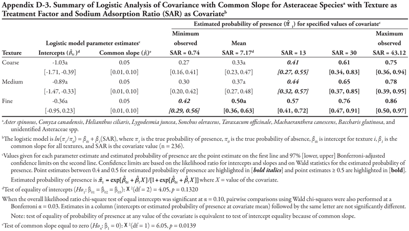
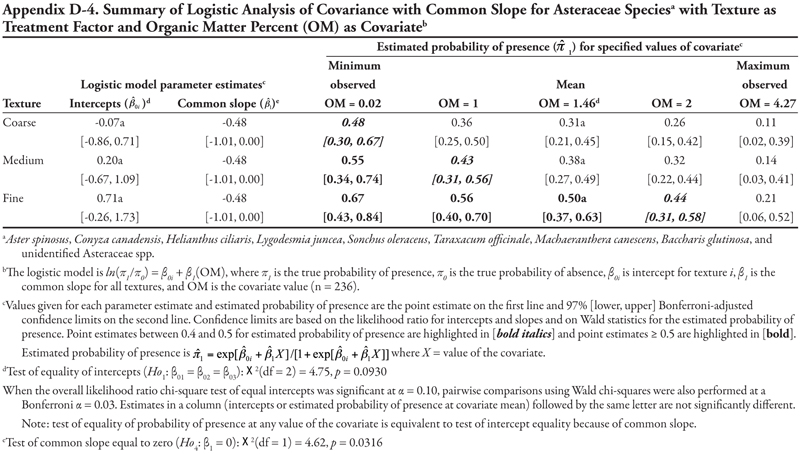
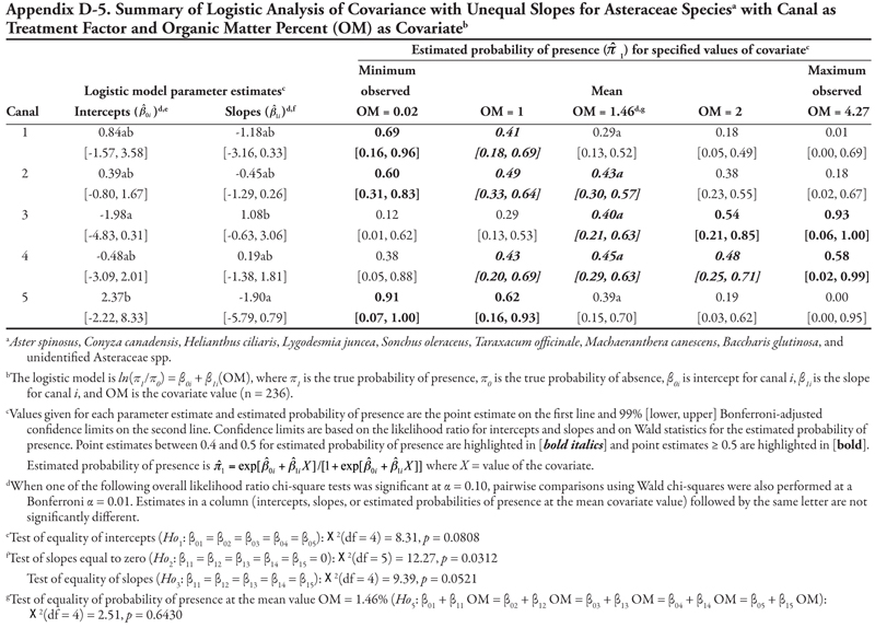
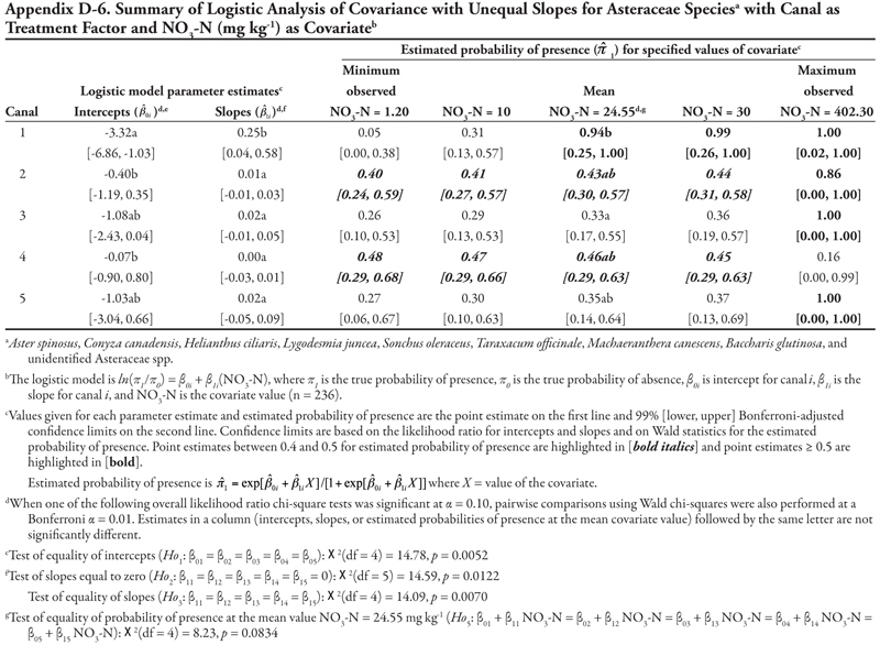

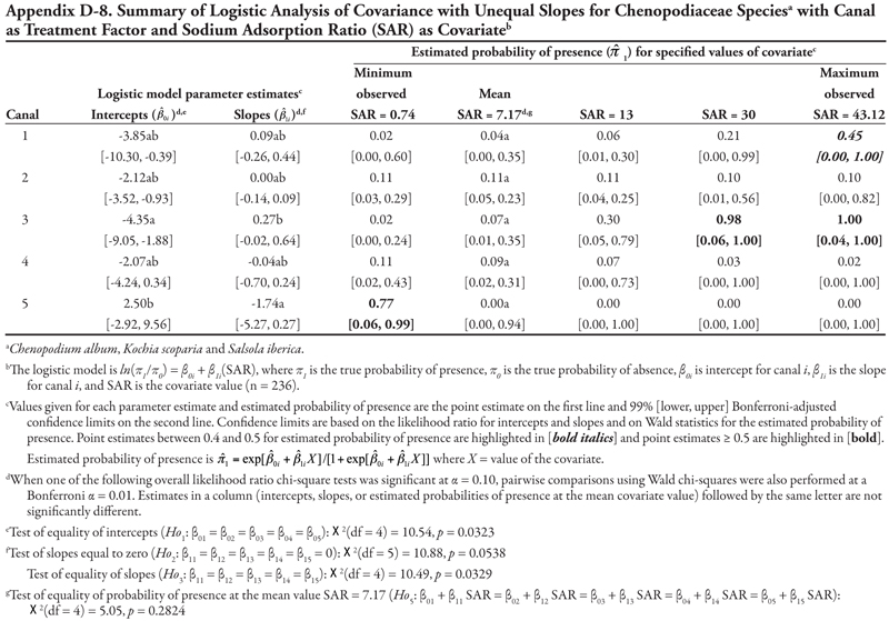
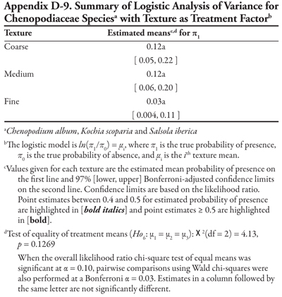
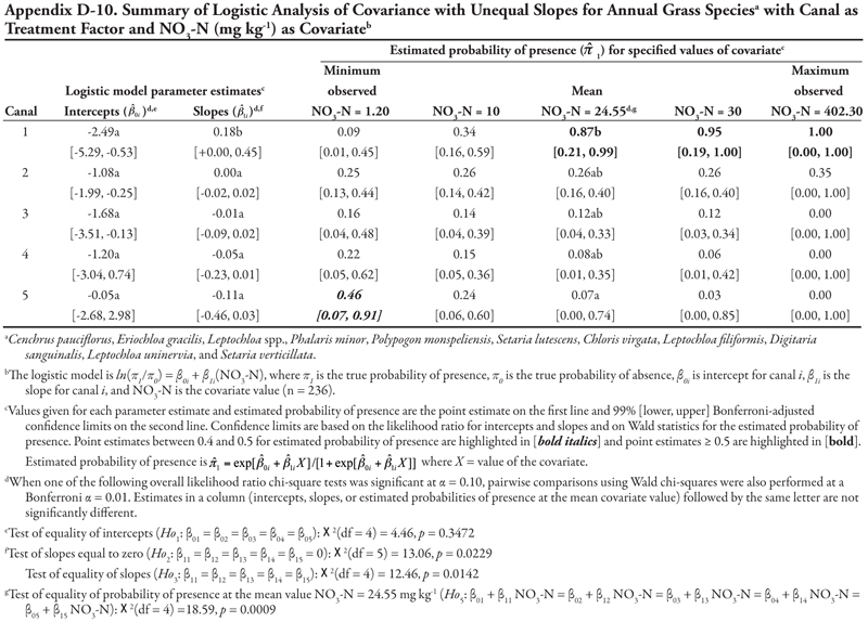
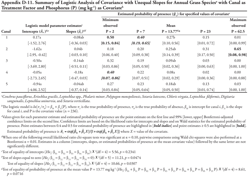
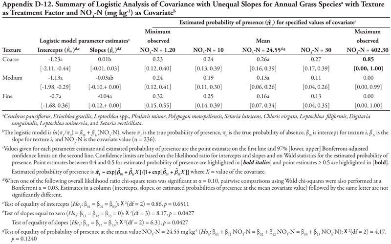
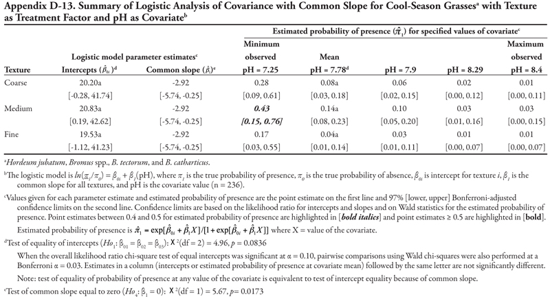
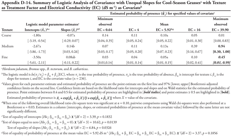
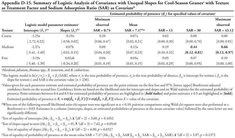
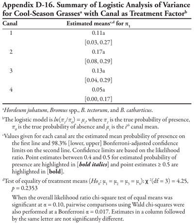
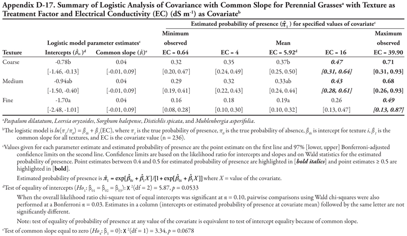
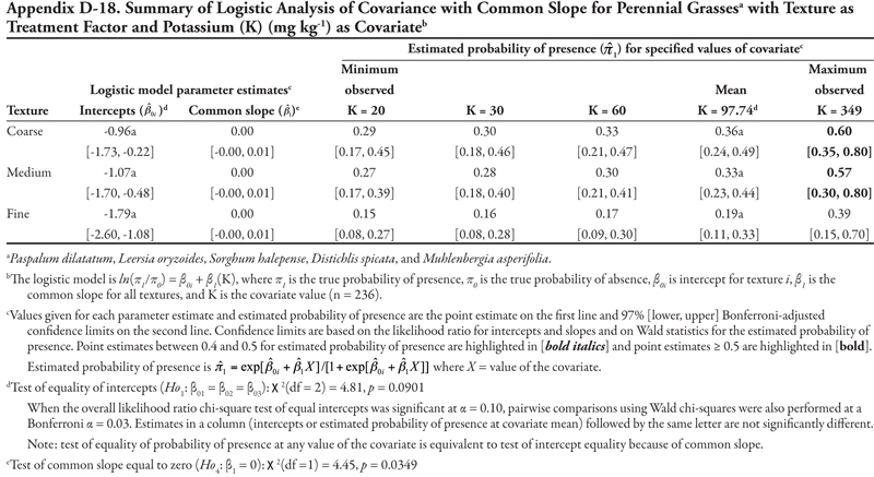
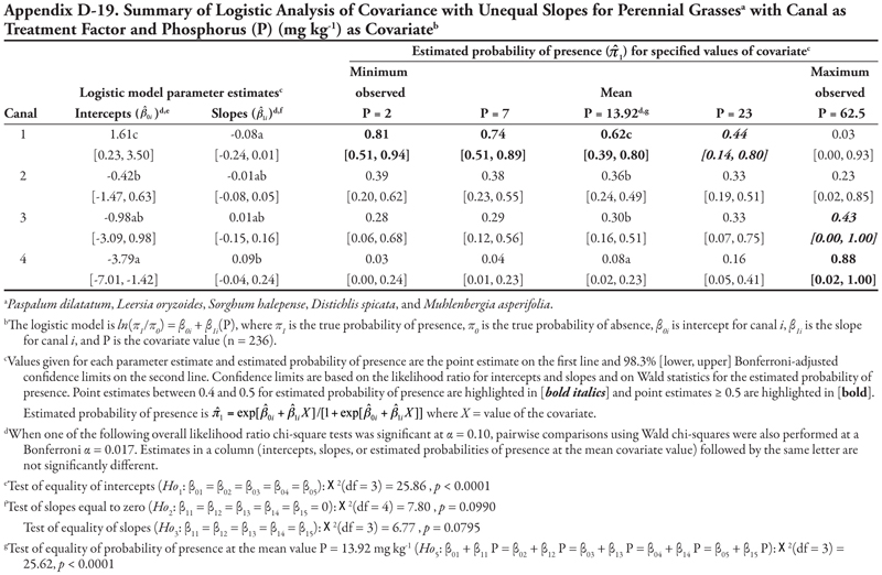
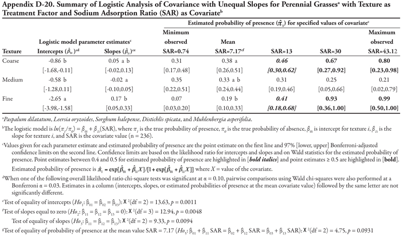
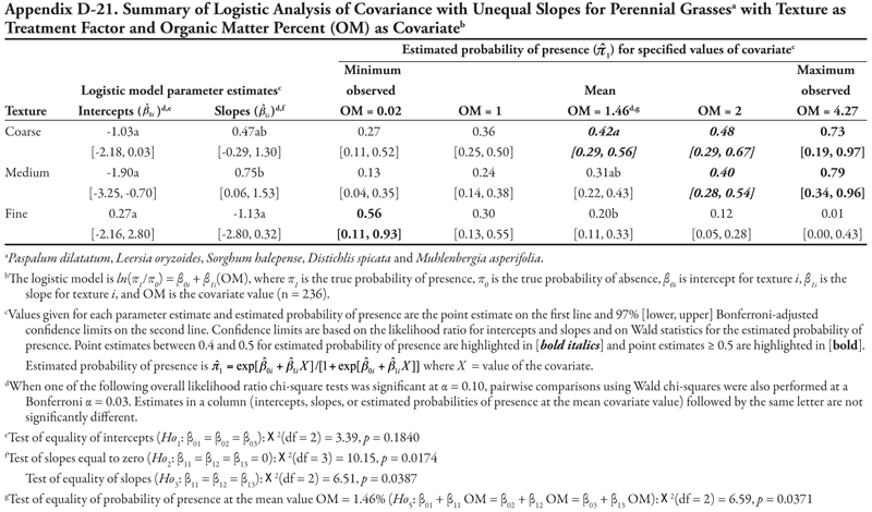
To find more resources for your business, home, or family, visit the College of Agricultural, Consumer and Environmental Sciences on the World Wide Web at aces.nmsu.edu.
Contents of publications may be freely reproduced for educational purposes. All other rights reserved. For permission to use publications for other purposes, contact pubs@nmsu.edu or the authors listed on the publication.
New Mexico State University is an equal opportunity/affirmative action employer and educator. NMSU and the U.S. Department of Agriculture cooperating.
Printed and electronically distributed on August 2012, Las Cruces, NM.